Building a document understanding pipeline with Google Cloud

Document understanding is the practice of using AI and machine learning to extract data and insights from text and paper sources such as emails, PDFs, scanned documents, and more. In the past, capturing this unstructured or “dark data” has been an expensive, time-consuming, and error-prone process requiring manual data entry. Today, AI and machine learning have made great advances towards automating this process, enabling businesses to derive insights from and take advantage of this data that had been previously untapped. 

In a nutshell, document understanding allows you to:

• Organize documents 
• Extract knowledge from documents 
• Increase processing speed

At Google Cloud we provide a solution, Document AI, which enterprises can leverage in collaboration with partners to implement document understanding. However, many developers have both the desire and the technical expertise to build their own document understanding pipelines on Google Cloud Platform (GCP)—without working with a partner—using the individual Document AI products.

If that sounds like you, this post will take you step-by-step through a complete document understanding pipeline. The Overview section explains how the pipeline works, and the step-by-step directions below walk you through running the code.

Overview

In order to automate an entire document understanding process, multiple machine learning models need to be trained and then daisy-chained together alongside processing steps into an end-to-end pipeline. This can be a daunting process, so we have provided sample code for a complete document understanding system mirroring a data entry workflow capturing structured data from documents.

Our example end-to-end document understanding pipeline consists of two components:

1. A training pipeline which formats the training data and uses AutoML to build Image Classification, Entity Extraction, Text Classification, and Object Detection models.
2. A prediction pipeline which takes PDF documents from a specified Cloud Storage Bucket, uses the AutoML models to extract the relevant data from the documents, and stores the extracted data in BigQuery for further analysis.

Training Data
The training data for this example pipeline is from a public dataset containing PDFs of U.S. and European patent title pages with a corresponding BigQuery table of manually entered data from the title pages. The dataset is hosted by the Google Public Datasets Project.

Part 1: The Training Pipeline

 The training pipeline consists of the following steps:

• Training data is pulled from the BigQuery public dataset. The training BigQuery table includes links to PDF files in Google Cloud Storage of patents from the United States and European Union.

• The PDF files are converted to PNG files and uploaded to a new Cloud Storage bucket in your own project. The PNG files will be used to train the AutoML Vision models.

• The PNG files are run through the Cloud Vision API to create TXT files containing the raw text from the converted PDFs. These TXT files are used to train the AutoML Natural Language models.

• The links to the PNG or TXT files are combined with the labels and features from the BigQuery table into a CSV file in the training data format required by AutoML. This CSV is then uploaded to a Cloud Storage bucket. Note: This format is different for each type of AutoML model.

• This CSV is used to create an AutoML dataset and model. Both are named in the format patent_demo_data_%m%d%Y_%H%M%S. Note that some AutoML models can sometimes take hours to train.

Part 2: The Prediction Pipeline

This pipeline uses the AutoML models previously trained by the pipeline above. For predictions, the following steps occur:

• The patent PDFs are collected from the prescribed bucket and converted to PNG and TXT files with the Cloud Vision API (just as in the training pipeline).

• The AutoML Image Classification model is called on the PNG files to classify each patent as either a US or EU patent. The results are uploaded to a BigQuery table.

• The AutoML Object Detection model is called on the PNG files to determine the location of any figures on the patent document. The resulting relative x, y coordinates of the bounding box are then uploaded to a BigQuery table.

• The AutoML Text Classification model is called on the TXT files to classify the topic of the patent content as medical technology, computer vision, cryptocurrency or other. The results are then uploaded to a BigQuery table.

• The AutoML Entity Extraction model is called to extract predetermined entities from the patent. The extracted entities are applicant, application number, international classification, filing date, inventor, number, publication date and title. These entities are then uploaded to a BigQuery table.

• Finally, the BigQuery tables above are joined to produce a final results table with all the properties above.

Step-by-Step Directions

For the developers out there, here’s how you can build the document understanding pipeline of your dreams. You can find all the code in our GitHub Repository.

Before you begin:

• You’ll need a Google Cloud project to run this demo. We recommend creating a new project.

• We recommend running these instructions in Google Cloud Shell (Quickstart). Other environments will work but you may have to debug issues specific to your environment. A Compute Engine VM would also be a suitable environment.

2. Install the necessary system dependencies. Note that in Cloud Shell system-wide changes do not persist between sessions, so if you step away while working through these step-by-step instructions you will need to rerun these commands after restarting Cloud Shell.

3. Create a virtual environment and activate it.

When your virtual environment is active you’ll see patents-demo-env in your command prompt. Note: If your Cloud Shell session ends, you’ll need to reactivate the virtual environment by running the second command again.

For the remaining steps, make sure you’re in the correct directory in the professional-services repo: /examples/cloudml-document-ai-patents/.

4. Install the necessary libraries into the virtual environment.

5. Activate the necessary APIs.

Note: We use the gcloud SDK to interact with various GCP services. If you are not working in Cloud Shell you’ll have to set your GCP project and authenticate by running gcloud init.

6. Edit the config.yaml file. Look for the configuration parameter project_id (under pipeline_project) and set the value to the project id where you want to build and run the pipeline. Make sure to enclose the value in single quotes, e.g. project_id: ‘my-cool-project’.

Note: if you’re not used to working in a shell, run nano to open a simple text editor.

7. Also in config.yaml, look for the configuration parameter creator_user_id (under service_acct) and set the value to the email account you use to log in to Google Cloud. Make sure to enclose the value in single quotes, e.g. creator_user_id: ‘cloud.user@fake.email.address.com’.

9. Run the training pipeline. This may take 3–4 hours, though some models will finish more quickly.

Note: If Cloud Shell Closes while the script is still downloading, converting, or uploading the PDFs, you will need to reactivate the virtual environment, navigate to the directory, and rerun the pipeline script. The image processing should take about 15-20 minutes, so make sure Cloud Shell doesn’t close during that time.

10. After training the models (wait about 4 hours), your Cloud Shell session has probably disconnected. Reconnect to Cloud Shell and run the following commands to reinstall dependencies, reactivate the environment, and navigate to the document understanding example code.

11. Next, you need to use the AutoML UIs to deploy the object detection and entity extraction models, and to find the ids of your models (which you will enter into config.yaml). In the UIs, you can also view relevant evaluation metrics about the model and see explicit examples where your model got it right (and wrong).

Note: Some AutoML products are currently in beta; the look and function of the UIs may change in the future.

Go to the AutoML Image Classification models UI, and make sure you are in same project you ran the training pipeline in (top right dropdown). Note the ID of your trained image classification model. Also note the green check mark to the right of the model—if this is not a check mark, or if there is nothing listed, it means model training is still in progress and you need to wait.

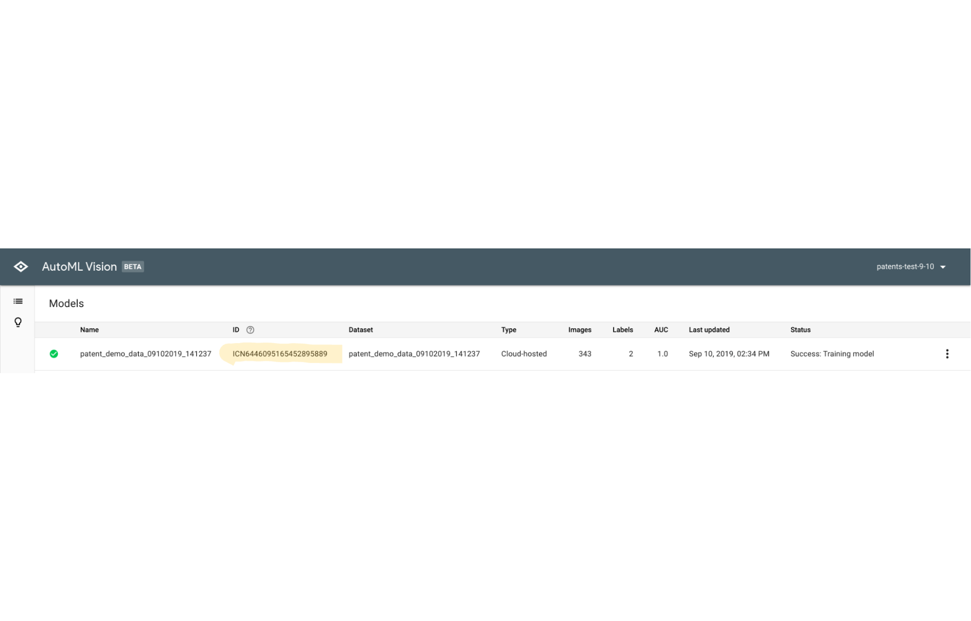
In Cloud Shell, edit config.yaml. Look for the line model_imgclassifier: and on the line below you’ll see model_id:. Put the image classification model id after model_id: in single quotes, so the line looks something like model_id: 'ABC1234567890'

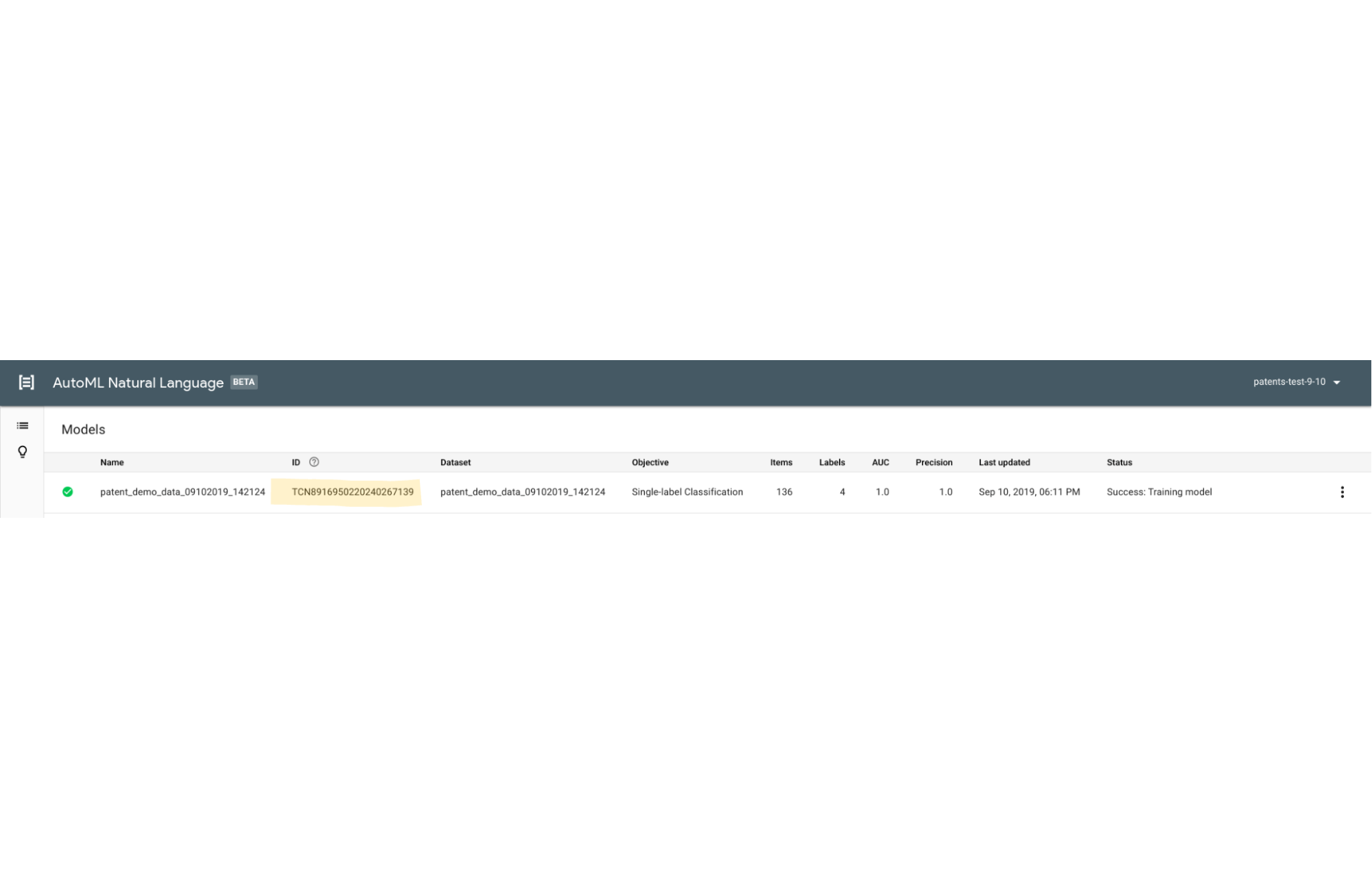
In Cloud Shell, edit config.yaml. Look for the line model_textclassifier: and on the line below you’ll see model_id:. Put the text classification model id after model_id: in single quotes, so the line looks something like " model_id: 'ABC1234567890'"

Go to the AutoML Object Detection models UI, again making sure your project is correct and your model is trained. In this UI, the model id is below the model name. 

You also need to deploy the model, by opening the menu under the three dots at the far right of the model entry and selecting “Deploy model”. A UI popup will ask how many nodes to deploy to, 1 Node is fine for this demo. You need to wait for the model to deploy before running prediction (about 10-15 minutes), the deployment status is in the UI under “Deployed” and it will be “Yes” when the model is deployed.

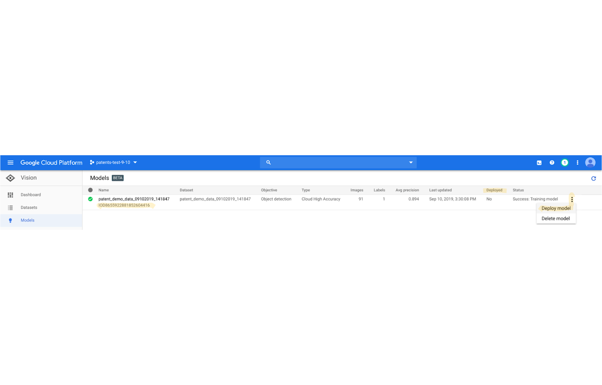
In Cloud Shell, edit config.yaml. Look for the line model_objdetect: and on the line below you’ll see model_id:. Put the object detection model id after model_id: in single quotes, so the line looks something like model_id: 'ABC1234567890'

To deploy the model, click the model name and a new UI view will open. Click “DEPLOY MODEL” near the top right and confirm. You need to wait for the model to deploy before running prediction (about 10-15 minutes), the UI will update when deployment is complete.

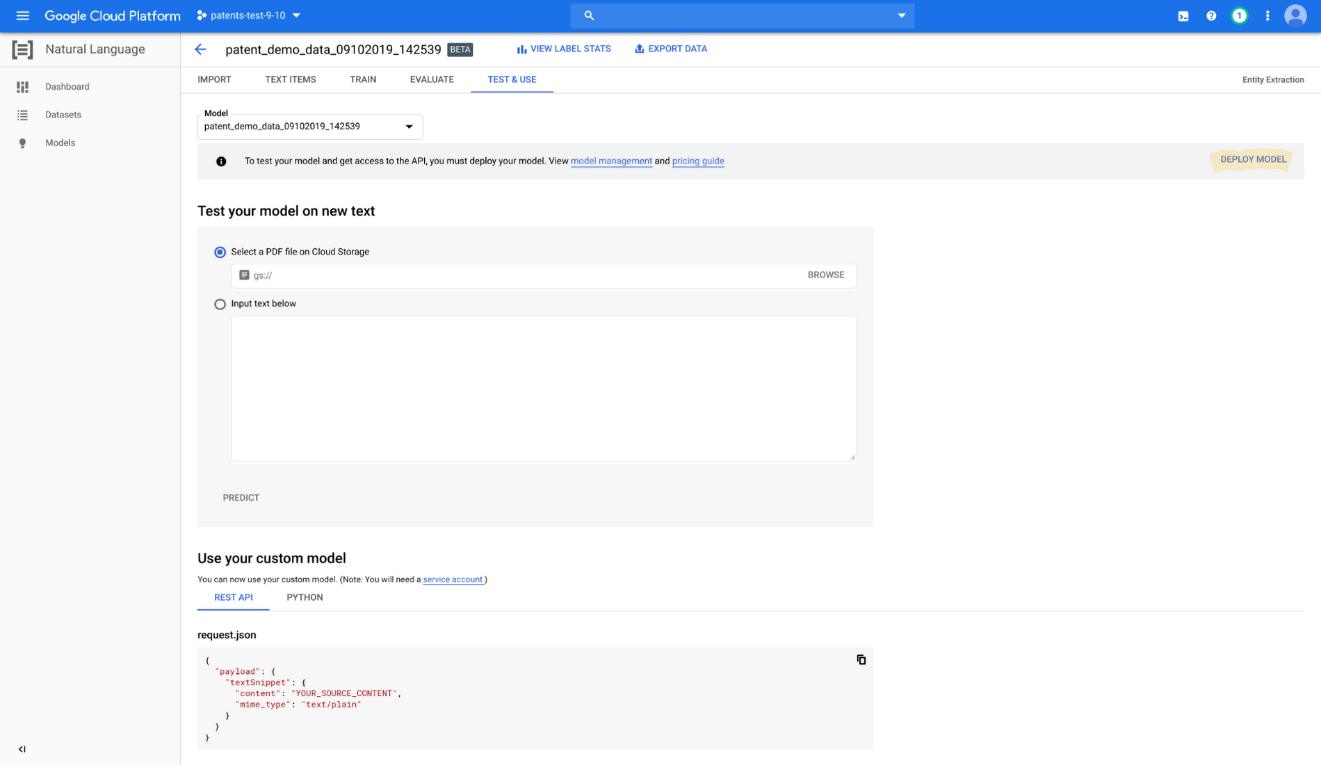
In Cloud Shell, edit config.yaml. Look for the line model_ner: and on the line below you’ll see model_id:. Put the entity extraction model id after model_id: in single quotes, so the line looks something like model_id: 'ABC1234567890'.

Before going further, make sure the model deployments are complete.

12. To run the prediction pipeline, you’ll need some PDFs of patent first pages in a folder in Cloud Storage. 

13. In the config.yaml file, fill in the configuration parameter labeled demo_sample_data (under pipeline_project) with the Cloud Storage location of the patents you want to process (in single quotes). If you’re following the example above, the parameter value is 'gs://<YOUR-PROJECT-ID>/patent_sample', substituting your project id.

Also, fill in the parameter labeled demo_dataset_id, just under demo_sample_data. With the BigQuery dataset (in single quotes) in your project where the predicted entities will be collected. For example, you can use 'patent_demo'. Note that this dataset must not exist already; the code will attempt to create the dataset and will stop running if the dataset already exists.

Now, you are ready to make predictions!

14. Run the prediction pipeline. This will process all the patent PDF first pages in the Cloud Storage folder specified in the demo_sample_data parameter, and upload predictions to (and create) BigQuery tables in the dataset specified by the  demo_dataset_id parameter.

python3 run_predict.py

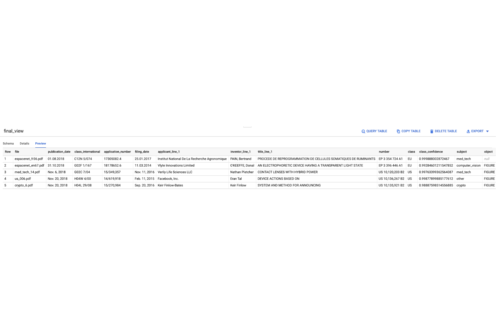
Note, for this, or any of the other intermediate tables that were created during the prediction pipeline, you may need to query the table to see the results since it is so new. For example:

If you are new to BigQuery, you can open a querying interface in the UI prepopulated with the table name by clicking the “QUERY TABLE” button visible when you select a table to view.

Conclusion

Congratulations! You now have a fully functional document understanding pipeline that can be modified for use with any PDF documents. To modify this example to work with your own documents, the data collection and training stages will need to be modified to pull documents from a local machine or another Cloud Storage bucket rather than a public BigQuery dataset. The training data will also need to be created manually for the specific type of documents you will be using. 

Now, if only we could create a robot that could scan paper documents to PDFs…