How to build demand forecasting models with BigQuery ML

Polong Lin
Developer Advocate
Retail businesses have a "goldilocks" problem when it comes to inventory: don't stock too much, but don't stock too little. With potentially millions of products, for a data science and engineering team to create multi-millions of forecasts is one thing, but to procure and manage the infrastructure to handle continuous model training and forecasting, this can quickly become overwhelming, especially for large businesses.
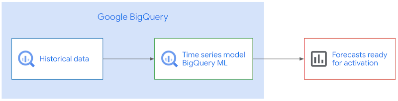
With BigQuery ML, you can train and deploy machine learning models using SQL. With the fully managed, scalable infrastructure of BigQuery, this means reducing complexity while accelerating time to production, so you can spend more time using the forecasts to improve your business.
So how can you build demand forecasting models at scale with BigQuery ML, for thousands to millions of products like for this liquor product below?
In this blogpost, I'll show you how to build a time series model to forecast the demand of multiple products using BigQuery ML. Using Iowa Liquor Sales data, I'll use 18 months of historical transactional data to forecast the next 30 days.
You'll learn how to:
- pre-process data into the correct format needed to create a demand forecasting model using BigQuery ML
- train an ARIMA-based time-series model in BigQuery ML
- evaluate the model
- predict the future demand of each product over the next n days
- take action on the forecasted predictions:
- create a dashboard to visualize the forecasted demand using Data Studio
- setup scheduled queries to automatically re-train the model on a regular basis
The data: Iowa Liquor Sales
The Iowa Liquor Sales data, which is hosted publicly on BigQuery, is a dataset that "contains the spirits purchase information of Iowa Class “E” liquor licensees by product and date of purchase from January 1, 2012 to current" (from the official documentation by the State of Iowa).
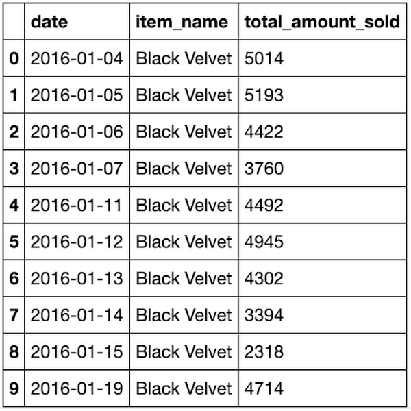
The raw dataset looks like this:
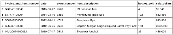
As on any given date, there may be multiple orders of the same product, we need to:
- Calculate the total # of products sold grouped by the date and the product
Cleaned training data
In the cleaned training data, we now have one row per date per item_name, the total amount sold on that day. This can be stored as a table or view. In this example, this is stored as bqmlforecast.training_data using CREATE TABLE.
Train the time series model using BigQuery ML
Training the time-series model is straight-forward.
How does time-series modeling work in BigQuery ML?
When you train a time series model with BigQuery ML, multiple models/components are used in the model creation pipeline. ARIMA, is one of the core algorithms. Other components are also used, as listed roughly in the order the steps they are run:
- Pre-processing: Automatic cleaning adjustments to the input time series, including missing values, duplicated timestamps, spike anomalies, and accounting for abrupt level changes in the time series history.
- Holiday effects: Time series modeling in BigQuery ML can also account for holiday effects. By default, holiday effects modeling is disabled. But since this data is from the United States, and the data includes a minimum one year of daily data, you can also specify an optional
HOLIDAY_REGION. With holiday effects enabled, spike and dip anomalies that appear during holidays will no longer be treated as anomalies. A full list of the holiday regions can be found in theHOLIDAY_REGIONdocumentation. - Seasonal and trend decomposition using the Seasonal and Trend decomposition using Loess (STL) algorithm. Seasonality extrapolation using the double exponential smoothing (ETS) algorithm.
- Trend modeling using the ARIMA model and the auto.ARIMA algorithm for automatic hyper-parameter tuning. In auto.ARIMA, dozens of candidate models are trained and evaluated in parallel, which include p,d,q and drift. The best model comes with the lowest Akaike information criterion (AIC).
Forecasting multiple products in parallel with BigQuery ML
You can train a time series model to forecast a single product, or forecast multiple products at the same time (which is really convenient if you have thousands or millions of products to forecast). To forecast multiple products at the same time, different pipelines are run in parallel.
In this example, since you are training the model on multiple products in a single model creation statement, you will need to specify the parameter TIME_SERIES_ID_COL as item_name. Note that if you were only forecasting a single item, then you would not need to specify TIME_SERIES_ID_COL. For more information, see the BigQuery ML time series model creation documentation.
Evaluate the time series model
You can use the ML.EVALUATE function (documentation) to see the evaluation metrics of all the created models (one per item):
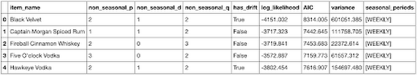
As you can see, in this example, there were five models trained, one for each of the products in item_name. The first four columns (non_seasonal_{p,d,q} and has_drift) define the ARIMA model. The next three metrics (log_likelihood, AIC, and variance) are relevant to the ARIMA model fitting process. The fitting process determines the best ARIMA model by using the auto.ARIMA algorithm, one for each time series. Of these metrics, AIC is typically the go-to metric to evaluate how well a time series model fits the data while penalizing overly complex models. As a rule-of-thumb, the lower the AIC score, the better. Finally, the seasonal_periods detected for each of the five items happened to be the same: WEEKLY.
Make predictions using the model
Make predictions using ML.FORECAST (syntax documentation), which forecasts the next n values, as set in horizon. You can also change the confidence_level, the percentage that the forecasted values fall within the prediction interval.
The code below shows a forecast horizon of "30", which means to make predictions on the next 30 days, since the training data was daily.
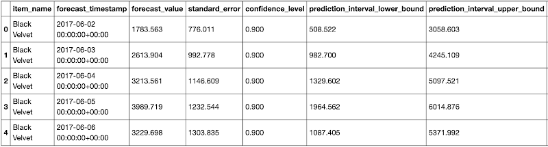
Since the horizon was set to 30, the result contains rows equal to 30 forecasted value * (number of items).
Each forecasted value also shows the upper and lower bound of the prediction_interval, given the confidence_level.
As you may notice, the SQL script uses DECLARE and EXECUTE IMMEDIATE to help parameterize the inputs for horizon and confidence_level. As these HORIZON and CONFIDENCE_LEVEL variables make it easier to adjust the values later, this can improve code readability and maintainability. To learn about how this syntax works, you can read the documentation on scripting in Standard SQL.
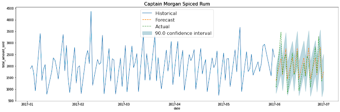
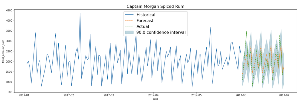
Plot the forecasted predictions
You can use your favourite data visualization tool, or use some template code here on Github for matplotlib and Data Studio, as shown below: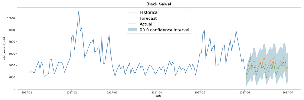
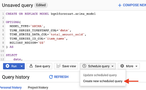
How do you automatically re-train the model on a regular basis?
If you're like many retail businesses that need to create fresh time-series forecasts based on the most recent data, you can use scheduled queries to automatically re-run your SQL queries, which includes your CREATE MODEL, ML.EVALUATE or ML.FORECAST queries.
1. Create a new scheduled query in the BigQuery UI
You may need to first "Enable Scheduled Queries" before you can create your first one.
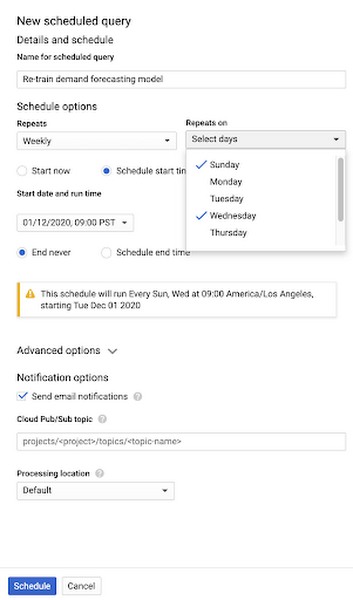
2. Input your requirements (e.g., repeats Weekly) and select "Schedule"
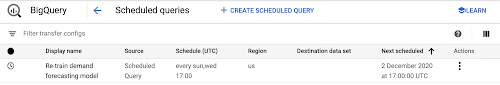
3. Monitor your scheduled queries on the BigQuery Scheduled Queries page
Extra tips on using time series with BigQuery ML
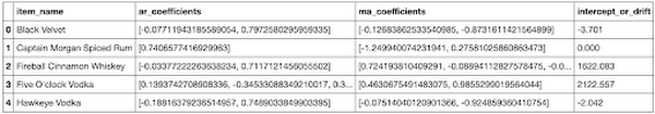
Inspect the ARIMA model coefficients
If you want to know the exact coefficients for each of your ARIMA models, you can inspect them using ML.ARIMA_COEFFICIENTS (documentation).
For each of the models, ar_coefficients shows the model coefficients of the autoregressive (AR) part of the ARIMA model. Similarly, ma_coefficients shows the model coefficients of moving-average (MA) part. They are both arrays, whose lengths are equal to non_seasonal_p and non_seasonal_q, respectively. The intercept_or_drift is the constant term in the ARIMA model.
Summary
Congratulations! You now know how to train your time series models using BigQuery ML, evaluate your model, and use the results in production.
Code on Github
You can find the full code in this Jupyter notebook on Github:
Join me on February 4 for a live walkthrough of how to train, evaluate and forecast inventory demand on retail sales data with BigQuery ML. I’ll also demonstrate how to schedule model retraining on a regular basis so your forecast models can stay up-to-date. You’ll have a chance to have their questions answered by Google Cloud experts via chat.
Want more?
I’m Polong Lin, a Developer Advocate for Google Cloud. Follow me on @polonglin or connect with me on Linkedin at linkedin.com/in/polonglin.
Please leave me your comments with any suggestions or feedback.
Thanks to reviewers: Abhishek Kashyap, Karl Weinmeister