History of massive-scale sorting experiments at Google

We’ve tested MapReduce by sorting large amounts of random data ever since we created the tool. We like sorting, because it’s easy to generate an arbitrary amount of data, and it’s easy to validate that the output is correct.

Even the original MapReduce paper reports a TeraSort result. Engineers run 1TB or 10TB sorts as regression tests on a regular basis, because obscure bugs tend to be more visible on a large scale. However, the real fun begins when we increase the scale even further. In this post I’ll talk about our experience with some petabyte-scale sorting experiments we did a few years ago, including what we believe to be the largest MapReduce job ever: a 50PB sort.

These days, GraySort is the large scale sorting benchmark of choice. In GraySort, you must sort at least 100TB of data (as 100-byte records with the first 10 bytes being the key), lexicographically, as fast as possible. The site sortbenchmark.org tracks official winners for this benchmark. We never entered the official competition.

MapReduce happens to be a good fit for solving this problem, because the way it implements reduce is by sorting the keys. With the appropriate (lexicographic) sharding function, the output of MapReduce is a sequence of files comprising the final sorted dataset.

Once in awhile, when a new cluster in a datacenter came up (typically for use by the search indexing team), we in the MapReduce team got the opportunity to play for a few weeks before the real workload moved in. This is when we had a chance to “burn in” the cluster, stretch the limits of the hardware, destroy some hard drives, play with some really expensive equipment, learn a lot about system performance, and, win (unofficially) the sorting benchmark.

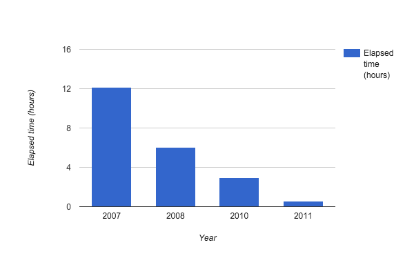
Figure 1: Google Petasort records over time.

2007: Our very first Petasort

We ran our very first Petasort in 2007. At that time, we were mostly happy that we got it to finish at all, although there are some doubts that the output was correct (we didn’t verify the correctness to know for sure). The job wouldn’t finish unless we disabled the mechanism which checks that the output of a map shard and its backup are the same. We suspect that this was a limitation of GFS (Google File System), which we used for storing the input and output. GFS didn’t have enough checksum protection, and sometimes returned corrupted data. Unfortunately, the text format used for the benchmark doesn’t have any checksums embedded for MapReduce to notice (the typical use of MapReduce at Google uses file formats with embedded checksums).

2008: The first time we focused on tuning

2008 was the first time we focused on tuning. We spent several days tuning the number of shards, various buffer sizes, prefetching/write-ahead strategies, page cache usage, etc. We blogged about the result here. The bottleneck ended up being writing the three-way replicated output to GFS, which was the standard we used at Google at the time. Anything less would have created a high risk of data loss.

2010

For this test, we used the new version of the GraySort benchmark that uses incompressible data. In the previous years, while we were reading/writing 1PB from/to GFS, the amount of data actually shuffled was only about 300TB, because the ASCII format used the previous years compresses well.

This was also the year of Colossus, the next generation distributed storage system at Google, the successor to GFS. We no longer had the corruption issues we encountered before with GFS. We also used Reed-Solomon encoding (a new Colossus feature) for output that allowed us to reduce the total amount of data written from 3 petabytes (for three-way replication) to about 1.6 petabytes. For the first time, we also validated that the output was correct.

To reduce the impact of stragglers, we used a dynamic sharding technique called reduce subsharding. This is the precursor to fully dynamic sharding used in Dataflow.

2011

This year we enjoyed faster networking and started to pay more attention to per-machine efficiency, particularly in I/O. We made sure that all our disk I/Os operations were performed in large 2MB blocks versus sometimes as small as 64kB blocks. We used SSDs for part of the data. That got us the first Petasort in under an hour — 33 minutes, to be exact — and we blogged about it here. We got really close (within 2x) to what the hardware was capable of given MapReduce’s architecture: input/output on a distributed storage, persisting intermediate data to disk for fault tolerance (and fault tolerance was important, because it would be common that some disks or even whole machines fail during an experiment at this scale).

We also scaled higher, and ran 10PB in 6 hours 27 minutes (26TB/min).

2012

For this test, we shifted our attention to running at a larger scale. With the largest cluster at Google under our control, we ran what we believe to be the largest MapReduce job ever in terms of amount of data shuffled. Unfortunately, the cluster didn’t have enough disk space for a 100PB sort, so we limited our sort to “only” 50PB. We ran it a single time and did so without specific tuning and we used the settings from our previous 10PB experiment. It finished in 23 hours, 5 minutes.

Note that this sort was 500 times larger than the GraySort large-scale requirement and twice as fast in throughput as the current 2015 official GraySort winner.

Lessons learned

While these sorting experiments are fun, they have several drawbacks:

1. Nobody really wants a huge globally-sorted output. We haven’t found a single use case for the problem as stated.

2. They show that the system is capable of performing well, although they de-emphasise how much effort it is. MapReduce needed a lot of tuning to perform this well. Indeed, we saw many MapReduce jobs in production that perform poorly due to what we would call misconfiguration.