Developing a JanusGraph-backed Service on Google Cloud
Ted Wilmes
By Ted Wilmes, Apache TinkerPop Project Management Committee
The graph database space is rapidly expanding as more and more companies identify potential use cases that require the traversal of highly connected network and hierarchical data sets in ways that are cumbersome with RDBMSs and NoSQL solutions. Today we’ll explore this graph database landscape with a focus on one of the popular open source options, JanusGraph. Then we’ll walk through the steps required to get a Java service up and running on Google Cloud Platform, accessing JanusGraph on a Cloud Bigtable cluster. JanusGraph is an Apache 2.0 licensed, Linux Foundation hosted graph database. Its roots trace back to the popular TitanDB, from which it forked in 2016.
If you’re new to graph databases, the learning curve can be steep. Before diving into JanusGraph specifics, let’s tackle one of the first questions users have when hearing about graph databases for the first time, “is my problem a graph problem?”
Is this a graph problem?
Let’s explore this question by first defining what we mean by graph. There are two graph modeling paradigms, Resource Description Framework (RDF) triplestores and property graphs. JanusGraph falls into the property graph category. Property graphs consist of vertices and edges (also referred to as nodes and relationships). Edges connect vertices to each other and are directed. These vertices and edges are labelled and can have properties. Property graph database providers diverge somewhat after that but this is a good mental model to get started. Triplestores take a different approach and provide a modeling paradigm that is based on triples. Triples take the form of subject-object-predicate. For example, Ted-uses-JanusGraph. We will not discuss triplestores any further in this blog post but they are quite powerful in their own right.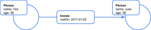
A sample property graph
Back to the question at hand, is my problem a graph problem? First, does the data that you’re attempting to store have one or more networks in it? Here are a few examples:
- Infrastructure monitoring: there is a prominent network created by all of the connections between the different components whether you’re monitoring industrial equipment in a factory or application instances running on GCP.
- Social networks: the canonical graph example where the network is created by communications and relationships between people.
- Finance: relationships arise from shared contact information and other pieces of customer metadata that identify members of the same business; certain financial instruments are composed of complex hierarchies of assets.
- Retail: though not directly connected to each other, customers become part of the retail network through their purchases of products.
- IoT: time series data is a big part of IoT, but great value can be derived from maintaining an accurate picture of the network of “things” being monitored including: identifying hidden dependencies and performing root cause analysis, and what downstream services will be affected by this switch going down?
- Finance: how is the value of this financial instrument derived from its complex structure of assets nested within assets?
- Project management: given a complex work breakdown structure, where are the bottlenecks in my process?
- SELECT name, age FROM persons
- SELECT name, age, address FROM persons INNER JOIN persons.id ON addresses.person_id
- SELECT year, month, qtr, SUM(sales) FROM company_earnings GROUP BY year, month, qtr
These examples demonstrate not only storage of networked data, but also dynamic, multi-hop traversals through that data. SQL recursive common table expressions (CTEs) and stored procedures can be written to address these uses if the data is kept in an RDBMS, but many users find the various property graph query languages, including Gremlin, a faster and more maintainable way to develop these queries.
Apache TinkerPop and JanusGraph
Property graph users have a number of options when it comes to not only graph database vendors, but also graph query languages. The Apache TinkerPop project provides one of these languages, Gremlin. In addition to Gremlin, TinkerProp includes a suite of components that property graph database providers can integrate into their own systems. This includes a distributed graph computation framework that runs on Spark, client drivers for Java, Javascript, Python, and .NET, and a server component, Gremlin Server, that enables remote graph access. Many different graph databases implement these APIs, JanusGraph being one of them.With so many options, why should a developer gravitate towards JanusGraph? One of the big draws beyond the up-to-date Gremlin support is JanusGraph’s support for pluggable storage and indexing. This provides the flexibility of running on a single instance—all the way up to a clustered deployment handling billions of nodes and edges, running on a distributed setup using Google Cloud Bigtable for persistence and Elasticsearch for fulltext and geospatial search. For this post, we’ll take the massive scale route and deploy JanusGraph over Cloud Bigtable and Elasticsearch on GCP.
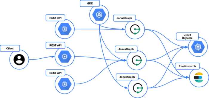
The JanusGraph architecture
Our example deployment will mimic a common production deployment pattern for JanusGraph. With Janus running separate from the storage and indexing backends. We will have two JanusGraph containers, running in the Google Kubernetes Engine, storing the graph data in a three-node Cloud Bigtable cluster, while using Elasticsearch for full text indexing and geospatial search. Our test client will connect to JanusGraph using the TinkerPop Java driver. Users typically increase or decrease their JanusGraph, storage layer, and indexing layer instance counts based upon their own performance requirements.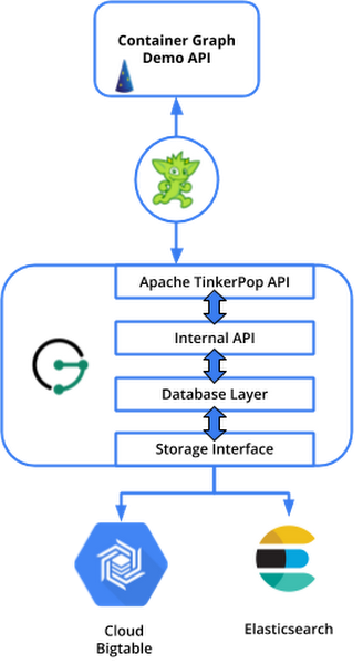
Deploying JanusGraph on GCP
You will need to start up a JanusGraph cluster prior to deploying the demo microservice for this post. Please refer to detailed instructions for deploying JanusGraph with Cloud Bigtable on GCP. After the JanusGraph cluster is running and healthy, return here to continue on to the development portion of this tutorial.The Scenario
Now that you have a JanusGraph cluster up and running, it’s time to deploy your first JanusGraph application. The app is a small Dropwizard microservice called Container Graph. Before we get into the code, let’s examine a use case that shows that a graph is worthwhile for this example.
Imagine Container Graph fitting into an existing ecosystem of services provided by a SaaS cloud monitoring company. They already have a service that ingests terabytes upon terabytes of time series data. There is an alarm service that stores alert rules and notifies affected parties when thresholds are breached and SLAs are broken. Recent user research has surfaced a new set of requirements. The current system does a good job of handling the components of their customers’ cloud deployments as isolated units, but our customers would like a more holistic view of how the pieces of their infrastructure are connected so that they can better plan for and address service issues. To start, when a service enters an alarm state, what other services may this affect even if they haven’t started alarming yet? Thinking back to our starter criteria, let’s see if we can check those boxes off. First, is there one or more networks in our data? Yes, the network arises from the connections between all of the running services. Second, will we need to make “graphy” queries? Yes, here too. Although there will be some basic CRUD methods to keep the graph up to date and retrieve basic details about the services, the heart of the customer request is a problem requiring traversals of networked data.
To this end, Container graph provides a number of REST endpoints to read and write data to a graph model of the infrastructure we just deployed to GKE. If you’re new to Dropwizard, it is a lightweight framework that makes it easy to develop RESTful applications so it’s a good fit for this example as the boilerplate is kept to a minimum.
Setup
You will need Java 8 and Maven to build and run this demo app. We’ll start things off by grabbing and building the code from here:
Deploy and test
Before deploying the Container Graph, you will need to get the IP address of the JanusGraph GKE internal load balancer with the following command:
If you’re running your Container Graph from the same instance you ran the last command, the Container Graph will use the $JANUSGRAPH_IP environment variable to connect. If you’re on a different instance, set JANUSGRAPH_IP to the load balancer IP address or open up the config.yml and change the contact point address to match the GKE load balancer’s internal address. Also be sure that the instance you run this example from has network access to the GKE cluster port 8182. To start the service, run:
Test that things are hooked up by retrieving a list of containers that we have stored in our graph:
The code
Now that the service is up and running, let’s walk through the graph-specific code. Keep in mind that even though this example uses Dropwizard, what you’ll be seeing, graph access-wise, is directly applicable to your other favorite frameworks.
Dependencies
Applications accessing JanusGraph remotely require two libraries. First, the TinkerPop Java driver, which is pulled in through the com.experoinc.dropwizard-tinkerpop dependency. dropwizard-tinkerpop is a small library that makes it easy to configure the TinkerPop driver in the Dropwizard environment. Second, you’ll need the janusgraph-core library. This library contains JanusGraph serializers that the driver uses to serialize and deserialize JanusGraph specific data types.
If you’re not using dropwizard-tinkerpop in your own projects, that dependency can be dropped and replaced with the TinkerPop Gremlin driver:
Always be mindful of what versions of JanusGraph and TinkerPop you’re using as the TinkerPop version should line up with the supported version for your JanusGraph deployment.
Making a connection
On startup, the application will create a driver connection to your graph. Connection configuration info is pulled in via dropwizard-tinkerpop and can be found in the config.yml file. Open up DeploymentGraphApplication.java, and you’ll see the following executed on application startup:
These lines allow your client to connect to the JanusGraph cluster using the configuration found in the config.yml and then creating a Gremlin GraphTraversalSource. You can think of this g as your connection to the remote graph. At this point, it is important to note that we’ll be using the Gremlin language embedded driver option, or in other words, writing our queries directly in Java. It is also possible to send string scripts to the server, one of the strongpoints when it comes to TinkerPop developer friendliness. Gremlin was a developed language embedded from the start and that is paying off now, allowing a very natural translation of the Gremlin syntax into other languages including Python and .NET. The drivers for these languages provide the same facilities. When a traversal is executed, it is serialized into Gremlin bytecode, which is then sent to the server for execution.
Graph schema
Our demo app checks to see if a schema exists, and if it does, data is loaded into the JanusGraph cluster when it starts up. Schema support varies across the different graph database providers. TinkerPop leaves schema management up to the graph provider so the schema creation syntax, though executed via the TinkerPop driver, is JanusGraph-specific.
The above snippet is an example of driver script submission using the client object. The mgmt object is an instance of the JanusGraph specific management interface. JanusGraph schema supports the definition of vertex and edge labels, property keys, indexes, and a variety of constraints.
Data loading
With a schema defined, the demo app will load a sample dataset representing our interconnected network of services, Cloud Bigtable, APIs, and client applications. Note that we have now switched over to vanilla Gremlin so we’re using the driver in language embedded mode. The below statement creates 50 client vertices and then the other vertices that represent our infrastructure. This single query hints at the expressiveness of the Gremlin language, even for pure mutation operations.
After the data is loaded, JanusGraph will be loaded with the data shown below.
The first query
Container Graph has a single resource class, ContainerGraphResource. This resource defines GET and POST methods to query and mutate our graph in a domain specific manner. The usual caveat applies here, that this is for demonstration purposes only and you likely would not embed your database access directly into your resource layer in a real application.
Let’s start with the simplest of queries, retrieving all of the containers that are deployed:
The GraphTraversalSource g has been injected into the resource via the resource constructor. As you continue your Gremlin journey, note that g is a commonly used convention when referencing the graph traversal source (an object that traversals are built off of).
Anatomy of a Gremlin traversal
Gremlin queries are called traversals, and those traversals are made of a series of steps. Each step falls into one of five categories: map, flat map, filter, side effect, and branch. Steps take arguments, and in many cases arguments can be other traversals. This ability to nest traversals within a traversal is an important tool and a requirement for writing powerful and concise Gremlin queries. We can break out simple first traversal down by step categorization as follows:
V(): This map step takes a graph as input, provided by the previous g and produces a stream of vertices. You may read this and think, a stream of all of the vertices in the graph, that sounds slow. However, like relational and other databases, graph databases have query optimizers: they take the input query and perform optimizations. As an example, these could include the usage of indexes, where applicable.hasLabel(“Container”): This filtering step, given the input stream of vertices, filters out all elements that do not have a label equal to “Container”valueMap(): this mapping step takes an element as its input and produces a stream of map objects consisting of the property key and values of the input elementtoList(): Though tacked on to the end of the traversal, this is not technically a Gremlin step. Traversals are lazily executed, so unless you iterate the traversal with atoList(),next(), or one of the other iterator methods, nothing will happen. This is a nice feature because it allows you to programmatically build traversals or break your large traversals out into chunks, which then can be later combined and executed.
Getting graphy with it
That first basic query, equivalent to a SELECT * FROM containers, wasn’t anything special. You’ll likely have a mixture of these basic CRUD type queries in your applications, but then as we discussed previously, the interesting portions of what you’re trying to do should exercise the networks in your data to make it a worthwhile graph effort. The remainder of the Container Graph resource has examples that move into this direction.
Let’s add a few steps to our toolbox that will allow us to reach out from our single vertex world to the surrounding graph.
out(): traverse outbound edges from the input vertexin(): navigate inbound edgesboth(): navigate both inbound and outbound edges
These steps are all flat map steps, taking a vertex as input and producing one more adjacent or incident vertices. Incidentally, they all optionally take a list of one or more labels as input to provide a filtering capability on which edges are followed.
We’ll nest a both() step inside of a repeat for our /container/{id}/connectedTo?hops={hops} endpoint:
The repeat step is a good sign that we’re starting to get graphy. At its most basic, the repeat step will loop over its internal traversal until it can no longer continue. For this query, a modulator step is added to repeat, times. Modulator steps are used throughout Gremlin to modify the behavior of parent steps. The times() step will limit the number of times repeat loops to the user-provided number of hops. A hops value of 1 will traverse both the inbound and outbound edges of the vertex with id = containerId and return the neighbors of this vertex. Two hops will produce a list of neighbors of these neighbors. The repeat is quite powerful and a step that you’ll need to become familiar with, so I recommend checking out the TinkerPop reference documentation for more details and modulator steps. The network of containers that we have stored may have containers that share neighbors with other containers, so a deduplication step is added that behaves like a DISTINCT in SQL by providing a list of unique elements given a list of elements that may contain duplicates.
Remember for a moment that this service is deployed alongside another infrastructure monitoring service that, given a stream of container metrics (CPU, memory, etc.), will generate alarms when said metrics exceed a preset threshold. As a user, it would be beneficial if I not only received the alarm, but also if I received a list of downstream services that may ultimately be affected by an outage of this container. By downstream we mean, we’re interested in the services that have this service as a dependency which is noted by a connectsTo edge. The /containers/{id}/downstream endpoint will do just that with the following Gremlin query:
Here, the both step is replaced with an in step since the query should only look at downstream services. The times modulator has been removed, and since we would like a list of all of the downstream services, an emit step is added that will produce the intermediate output of the repeat at each iteration. Here’s an example of what the results will look like if one of the Elasticsearch instances has issues:
More advanced data projection
Taking what we’ve learned so far, let’s look at one more traversal that calculates a simple statistic for each container. This query adds a very powerful new step, project, and makes use of a modulating by step with an order. Before jumping down to the explanation, take a look and see if you can determine what output this will produce.
The project step takes vertices as input here, specifically labelled as containers due to the previous hasLabel output. We’ve only shown examples with vertices and edges so far, but many of the Gremlin steps can operate on collections including maps and lists in addition to graph elements. The project step defines a transformation from its input into a stream of maps. The arguments define which keys will be present in the output map and each “by” modulating step defines the mapping that will produce the value for its respective key.
The first "by", by(“containerId”) returns the containerId property value, mapping it to the containerId property in the output map. The second "by" is much more interesting: here we nest one of the repeat traversals. For each container vertex coming into the project, we will produce a map with a container id. The result of the repeat traversal is a count of the direct and transitive dependencies of each container. This is a process in which, in terms of expressivity, Gremlin starts to shine.
Finally, given the stream of maps returned by the project, the order step sorts them in descending order by the value of the dependency count.
There are a number of other query examples in the project that aren’t covered here, including the graph mutation operations, that I encourage you to look at to continue your Gremlin journey. All of the queries can also be run from the Gremlin console. Sometimes it is helpful to break more complex queries down into chunks, running smaller portions independently and interactively in the console to better understand how each step is working.
Next steps
Over the course of this post, we’ve learned about Apache TinkerPop, JanusGraph, and deployed a microservice to connect to a two-node JanusGraph cluster. With this setup in place, you can begin further experimentation, and perhaps start to build out your first JanusGraph-based application. Stay tuned in to janusgraph.org and the JanusGraph user group for the latest in JanusGraph news. Help and general discussion can also be found on the JanusGraph Gitter channel. For further details on Gremlin, I highly recommend Kelvin Lawrence’s ever expanding Practical Gremlin: An Apache TinkerPop Tutorial along with the authoritative TinkerPop reference documentation.
If you’re headed to the upcoming Google Next ‘18 we’ll be presenting JanusGraph on Cloud Bigtable use cases in the IoT, financial services, and supply chain spaces.
Acknowledgements
Special thanks to Sami Zuhuruddin for developing the JanusGraph Helm chart and detailed deployment instructions