Scaling heterogeneous graph sampling for GNNs with Google Cloud Dataflow
Brandon Mayer
Senior Software Engineer
Bryan Perozzi
Research Scientist
This blog presents an open-source solution to heterogeneous graph sub-sampling at scale using Google Cloud Dataflow (Dataflow). Dataflow is Google’s publicly available, fully managed environment for running large scale Apache Beam compute pipelines. Dataflow provides monitoring and observability out of the box and is routinely used to scale production systems to easily handle extreme datasets.
This article will present the problem of graph sub-sampling as a pre-processing step for training a Graph Neural Network (GNN) using Tensorflow-GNN (TF-GNN), Google’s open-source GNN library.
The following sections will motivate the problem, present an overview of the necessary tools including Docker, Apache Beam, Google Cloud Dataflow, TF-GNN Unigraph format, TF-GNN graph-sampler concluding with end-to-end tutorial using large heterogeneous citation network (OGBN-MAG) popular for GNN (node-prediction) benchmarking. We do not cover modeling or training with TF-GNN which is covered by the libraries’ documentation and paper.
Motivation
Relational datasets (datasets with graph structure) including data derived from social graphs, citation networks, online communities and molecular data continue to proliferate and applying Deep Learning methods to better model and derive insights from structured data are becoming more common. Even if a dataset is originally unstructured, it’s not uncommon to observe performance gains for ML tasks by inferring structure before applying deep learning methods through tools such as Grale (semi-supervised graph learning).
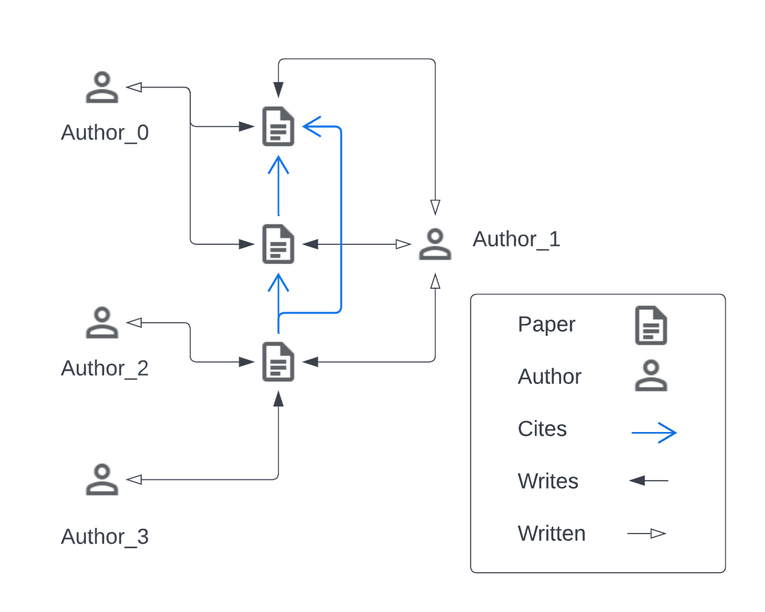
Visualized below is a synthetic example visualizing a citation network in the same style as the popular OGBN-MAG dataset. The figure shows a heterogeneous graph - a relational dataset with multiple types of nodes (entities) and relationships (edges) between them. In the figure there are two entities, “Paper” and “Author”. Certain authors “Write” specific papers defining a relation between “Author” entities and “Paper” entities. “Papers” commonly “cite” other “Papers” building a relationship between the “Paper” entities.
For real world applications, the number of entities and relationships may be very large and complex and in most cases, it is impossible to load a complete dataset into memory on a single machine.
Graph Neural Networks (GNNs or GCNs) are a fast growing suite of techniques for extending Deep Learning and Message Passing frameworks to structured data and Tensorflow GNN (TF-GNN) is Google’s Graph Neural Networks library built on the Tensorflow platform. TF-GNN defines native tensorflow objects, including tfgnn.GraphTensor, capable of representing arbitrary heterogeneous graphs, models and processing pipelines that can scale from academic to real world applications including graphs with millions of nodes and trillions of edges.
Scaling GNN models to large graphs is difficult and an active area of research as real world structured data sets typically do not fit in the memory available on a single computer making training/inference using a GNN impossible on a single machine. A potential solution is to partition a large graph into multiple pieces, each of which can fit on a single machine and be used in concert for training and inference. As GNNs are based on message-passing algorithms, how the original graph is partitioned is crucial to model performance.
While conventional Convolutional Neural Networks (CNNs) have regularity that can be exploited to define a natural partitioning scheme, kernels used to train GNNs potentially overlap the surface of the entire graph, are irregularly shaped and are typically sparse. While other approaches to scaling GCNs exist, including interpolation and precomputing aggregations, we focus on subgraph sampling: partitioning the graph into smaller subgraphs using random explorations to capture the structure of the original graph.
In the context of this document, the graph sampler is a batch Apache Beam program that takes a (potentially) large, heterogeneous graph and a user-supplied sampling specification as input, performs subsampling, and writes tfgnn.GraphTensors to a storage system encoded for downstream TF-GNN training.
Introduction to Docker, Beam, and Google Cloud Dataflow
Apache Beam (Beam) is an open-source SDK for expressing compute intensive processing pipelines with support for multiple backend implementations. Google Cloud Platform (GCP) is Google’s cloud computing service, of which Dataflow is GCPs implementation for running Beam pipelines at scale. The two main abstractions defined by the Beam SDK are
Pipelines - computational steps expressed as a DAG (Directed Acyclic Graph)
Runners - Environments for running pipelines using different types of controller/server configurations and options
Computations are expressed as Pipelines using the Apache Beam SDK and the Runners define a compute environment. Specifically, Google provides a Beam Runner implementation called the DataflowRunner that connects to a GCP project (with user supplied credentials) and executes the Beam pipeline in the GCP environment.
Executing a Beam pipeline in a distributed environment involves the use of “worker” machines, compute units that execute steps in the DAG. Custom operations defined using the Beam SDK must be installed and available on the worker machines and data communicated between workers must be able to be serialized/deserialized for inter-worker communication. In addition to the DataflowRunner, there exists a DirectRunner which enables users to execute Beam pipelines on local hardware and is typically used for development, verification, and testing.
When clients use the DirectRunner to launch Beam pipelines, the compute environment of the pipeline mirrors the local host; libraries and data available on the users’ machine are available to the Beam work units. This is not the case when running in a distributed environment. Worker machines compute environments are potentially different from the host that dispatches the remote Beam pipeline. While this might be sufficient for Pipelines that only rely on python standard libraries, this is typically not acceptable for scientific computing which may rely on mathematical packages or custom definitions and bindings.
For example, TFGNN defines Protocol Buffers (tensorflow/gnn/proto) whose definitions must be installed both on the client that initiates the Beam pipeline and the workers that execute the steps of the sampling DAG. One solution is to generate a Docker image that defines a complete TFGNN runtime environment that can be installed on Dataflow workers before Beam pipeline execution.
Docker containers are widely used and supported in the open source community for defining portable virtualized run-time environments that can be isolated from other applications on a common machine. A Docker Container is defined as a running instance of a Docker Image (conceptually a read-only binary blob or template). Images are defined by a Dockerfile that enumerates the specifics of a desired compute environment. Users of a Dockerfile “build” a Docker Image which can be used and shared by other people who have Docker installed to instantiate the isolated compute environment. Docker images can be built locally with tools like the Docker CLI or remotely via Google Cloud Build (GCB). Docker images can be shared in public or private repositories such as Google Container Registry or Google Artifact Registry.
TF-GNN provides a Dockerfile specifying an operating system along with a series of packages, versions and installation steps to set up a common, hermetic compute environment that any user of TF-GNN (with docker installed) can use. With GCP, TF-GNN users can build a TF-GNN docker image and push that image to an image repository that Dataflow workers can install prior to being scheduled by a Dataflow pipeline execution.
Unigraph Data Format
The TF-GNN graph sampler accepts graphs in a format called unigraph. Unigraph supports very large, homogeneous and heterogeneous graphs with variable numbers of node sets and edge sets (types). Currently, in order to use the graph sampler, users need to convert their graph to unigraph format.
The unigraph format is backed by a text-formatted GraphSchema protocol buffer (proto) message file describing the full (unsampled) graph topology. The GraphSchema defines three main artifacts:
context: Global graph features
node sets: Sets of nodes with different types and (optionally) associated features
edge sets: the directed edges relating nodes in node sets
For each context, node set and edge set there is an associated “table” of ids and features which may be in one of many supported formats; CSV files, shared tf.train.Example protos in TFRecords containers and more. The location of each “table” artifact may be absolute or local to the schema. Typically, a schema and all “tables” live under the same directory which is dedicated to the graph’s data.
Unigraph is purposefully simple to enable users to easily translate their custom data source into a unigraph format which the graph sampler and subsequently TF-GNN can consume.
Once the unigraph is defined, the graph sampler requires two more configuration artifacts:
(Optional) Seed node-ids
If provided, random explorations will begin from the specified “seed” node-ids only.
The graph sampler generates subgraphs by randomly exploring the graph structure starting from a set of “seed nodes”. The seed nodes are either explicitly specified by the user or, if omitted, every node in the graph is used as a seed node which will result in one subgraph for every node in the graph. Exploration is done at scale, without loading the entire graph on a single machine through the use of the Apache Beam programming model and Dataflow engine.
A SamplingSpec message is a graph sampler configuration that allows the user control how the sampler will explore the graph through edge sets and perform sampling on node sets (starting from seed nodes). The SamplingSpec is yet another text formatted protocol buffer message that enumerates sampling operations starting from a single `seed_op` operation.
Example: OGBN-MAG Unigraph Format
As a clarifying example, consider the OGBN-MAG dataset, a popular, large, heterogeneous citation network containing the following node and edge sets:
OGBN-MAG Node Sets
"paper" contains 736,389 published academic papers, each with a 128-dimensional word2vec feature vector computed by averaging the embeddings of the words in its title and abstract.
"field_of_study" contains 59,965 fields of study, with no associated features.
"author" contains the 1,134,649 distinct authors of the papers, with no associated features
"institution" contains 8740 institutions listed as affiliations of authors, with no associated features.
OGBN-MAG Edge Sets
"cites" contains 5,416,217 edges from papers to the papers they cite.
"has_topic" contains 7,505,078 edges from papers to their zero or more fields of study.
"writes" contains 7,145,660 edges from authors to the papers that list them as authors.
"affiliated_with" contains 1,043,998 edges from authors to the zero or more institutions that have been listed as their affiliation(s) on any paper.
This dataset can be described in unigraph with the following skeleton GraphSchema message:
Example OBGN-MAG unigraph GraphSchema protocol buffer message.
This schema omits some details (a full example is included in the TFGNN repository) but the outline is sufficient to show that the GraphSchema message merely enumerates the node types as collections of node_sets and the relationships between the node sets are defined by the edge_sets messages.
Note the additional “written” edge set. This relation is not defined in the original dataset or manifested on persistent media. However, the “written” table specification defines a reverse relation creating a directed edge from papers back to authors as the transpose of the “writes” edge set. The tfgnn-sampler will parse the metadata.extra tuple and if the edge_type/reverse key-value pair is present, generate an additional PCollection of edges (relations) that swaps the sources and targets relative the relations expressed on persistent media.
Sampling Specification
A TF-GNN modeler would craft a SamplingSpec configuration for a particular task and model. For OGBN-MAG, one particular task is to predict the venue (journal or conference) that a paper from a test set is published at. The following would be a valid sampling specification for that task:
A valid SamplingSpec configuration for the OGBN-MAG venue prediction challenge.
This particular SamplingSpec may be visualized in plate notation showing the relationship between the node sets and relations in the sampling specification as:
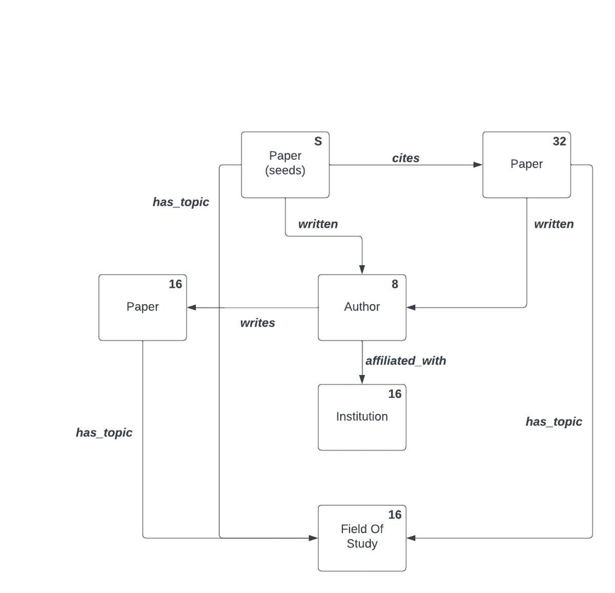
In human-readable terms, this sampling specification may be described as the following sequence of steps:
Use all entries in the "papers" node set as "seed" nodes (roots of the sampled subgraphs).
Sample 16 more papers randomly starting from the "seed" nodes through the citation edge set. Call this sampled set "seed->paper".
For both the "seed" and "seed->paper" sets, sample 8 authors using the "written" edge set. Name the resulting set of sampled authors "paper->author".
For each author in the "paper->author" set, sample 16 institutions via the "affiliated_with" edge set.
For each paper in the "seed", "seed->paper" and "author->paper" sample 16 fields of study via the "has_topic" relation.
Node vs. Edge Aggregation
Currently, the graph sampler program takes an optional input flag edge_aggregation_method which can be set to either node or edge (defaults to edge). The edge aggregation method defines the edges that the graph sampler collects on a per-subgraph basis after random exploration.
Using the edge aggregation method, the final subgraph will only include the edges traversed during random exploration. Using the node aggregation method, the final subgraph will contain all edges that have a source and target node in the set of nodes visited during exploration.
As a clarifying example, consider a graph with three nodes {A, B, C} with directed edges as shown below.
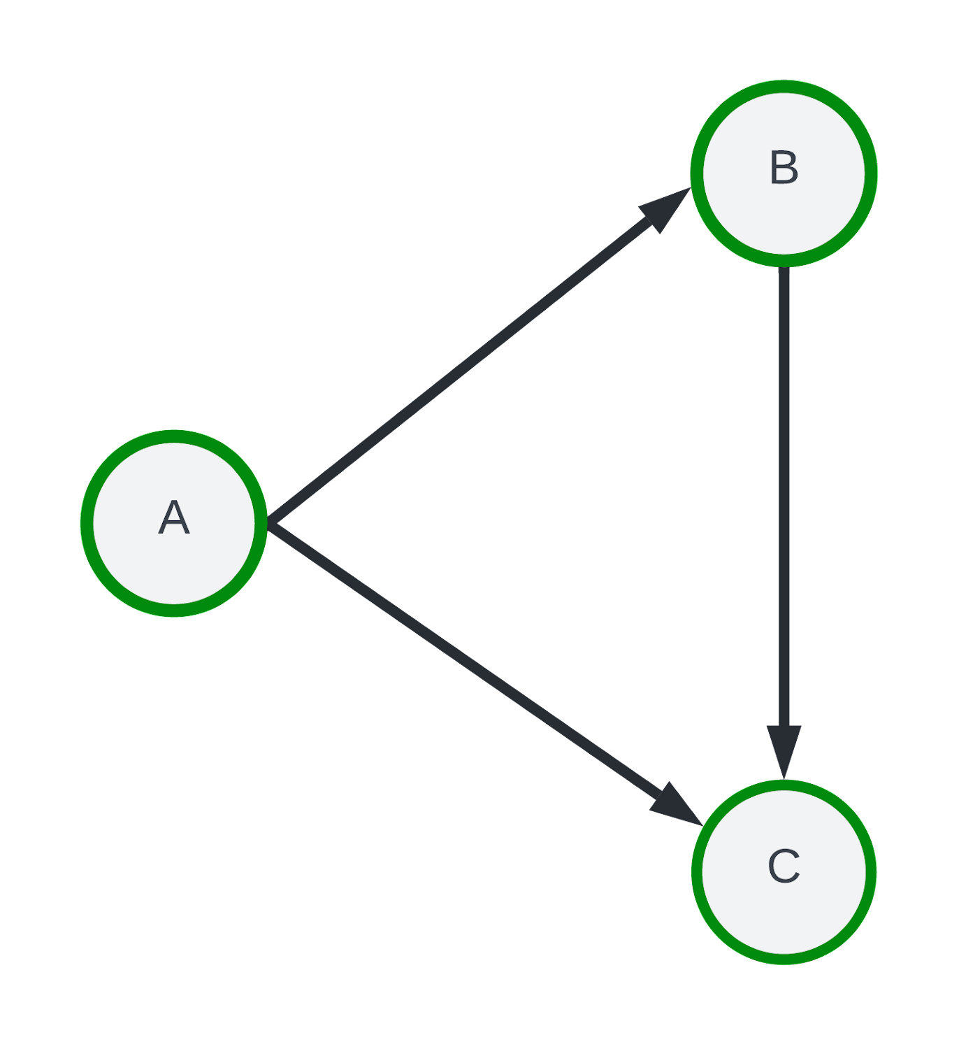
Instead of random exploration, assume we perform a one-hop breadth first search exploration starting at seed-node “A”, traversing edges A → B and A → C. Using the edge aggregation method, the final subgraph would only retain edges A → B and A → C while the node aggregation would include A → B, A → C and the B → C edge. The example sampling paths along with the edge and node aggregation results are visualized below.
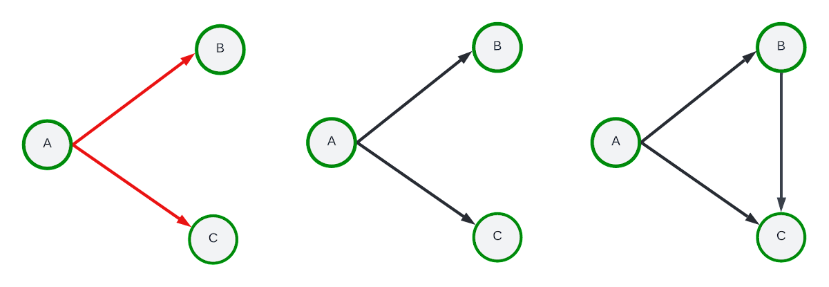
Right: Node aggregation sampling result.
The edge aggregation method is less expensive (time and space) than node aggregation yet node aggregation typically generates subgraphs with higher edge density. It has been observed in practice that node-based aggregation can generate better models during training and inference for some datasets.
TF-GNN Graph Sampling with Google Cloud Dataflow OBGN-MAG: End-To-End Example
While alternative workflows are possible, this tutorial assumes the user will be building Docker images and initiating a Dataflow job from a local machine with internet access.
First install docker on a local host machine then checkout the tensorflow_gnn repository.
The user will need the name of their GCP project (which we refer to as GCP_PROJECT) and some sort of GCP credentials. Default application credentials are typical for developing and testing within an isolated project but for production systems, consider maintaining custom service account credentials. Default application credentials may be obtained by:
On most systems, this command will download the access credentials to the following location: ~/.config/gcloud/application_default.json.
Assuming the location of the cloned TF-GNN repository is ~/gnn, The TF-GNN docker image can be built and pushed the a GCP container registry with the following:
Building and pushing the image may take some time. To avoid the local build/push, the image can be built directly from a local Dockerfile remotely using Google Cloud Build.
Get the OGBN-MAG Data
The TFGNN repository has a ~/gnn/examples directory containing a program that will automatically download and format common graph datasets from the OGBN website as unigraph. The shell script ./gnn/examples/mag/download_and_format.sh will execute a program in the docker container and download the ogbn-mag dataset to /tmp/data/ogbn-mag/graph on your local machine and convert it to unigraph resulting in the necessary GraphSchema and sharded TFRecord files representing the node and edge sets.
To run sampling at scale with Dataflow on GCP, we’ll need to copy this data to a Google Cloud Storage (GCS) bucket so that Dataflow workers have access to the graph data.
Launching TF-GNN Sampling on Google Cloud Dataflow
At a high level, the process of pushing a job to Dataflow using a custom Docker container may be visualized as follows:
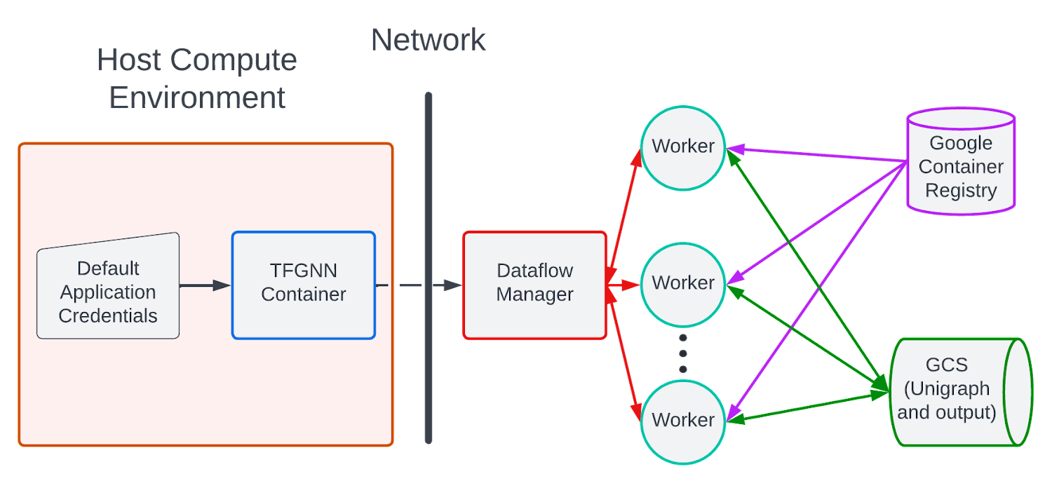
A user builds the TF-GNN docker image on their local machine, pushes the docker image to their GCR repository and sends a pipeline specification to the GCP Dataflow service. When the pipeline specification is received by the GCP Dataflow service, the pipeline is optimized, Dataflow workers (GCP VMs) are instantiated and pull and run the TF-GNN image that the user pushed to GCR.
The number of workers automatically scale up/down according to the Dataflow autoscaling algorithm which by default monitors pipeline stage throughput. The input graph is hosted on GCP and the sampling results (GraphTensor output) are written to sharded *.tfrecord files on Google Cloud Storage.
This process can be instantiated by filling in some variables and running the script: ./gnn/tensorflow_gnn/examples/mag/sample_dataflow.sh.
These environment variables specify the GCP project resources and the location of inputs required by the Beam sampler.
The TEMP_LOCATION variable is a path that is needed by Dataflow workers for shared scratch space and the samples are finally written to sharded TFRecord files at $OUTPUT_SAMPLES (a GCS location). REMOTE_WORKER_CONTAINER must be changed to the appropriate GCR URI pointing to the custom TF-GNN image.
GCP_VPN_NAME is a variable holding a GCP network name. While the default VPC will work, the default network allocates Dataflow worker machines with IPs that have access to the public internet. These types of IPs count against GCP “in-use” IP quota range. As Dataflow worker dependencies are shipped in the Docker container, workers do not need IPs with external internet access and setting up a VPC without external internet access is recommended. See here for more information. To use the default network, set GCP_VPN_NAME=default and remove --no_use_public_ips from the command below.
The main command to start the Dataflow tfgnn-sampler job follows:
This command mounts the users default application credentials, sets the $GOOGLE_CLOUD_PROJECT and $GOOGLE_APPLICATION_CREDENTIALS in the container runtime, launches the tfgnn_graph_sampler binary and sends the sampler DAG to the Dataflow service. Dataflow workers will fetch their runtime environment from the tfgnn:latest image stored in GCR and the output will be placed on GCS in the $OUTPUT_SAMPLES location, ready to train a TF-GNN model.