Price optimization notebook for apparel retail using Google Vertex AI

Accurate demand forecasting and intelligent demand correction through price changes and promotions are common in many industries like retail, consumer goods, travel and manufacturing. Google Cloud and Grid Dynamics teamed up to develop a reference price optimization pipeline in Vertex AI, Google Cloud’s data science platform. This starter kit is built upon best practices developed by Grid Dynamics from multiple real-world price optimization projects with leading retail, manufacturing, and CPG customers. It leverages the state-of-the-art AutoML forecasting model from Vertex AI Forecast and shows how to find optimal price points for every product to maximize profit. 

Situation and Challenge

The product prices often change based on the observed market response, sell-through rates, supply disruptions, and other factors. Rule based or manual price management in spreadsheets doesn’t scale well to large catalogs with thousands of items. These methods are slow, error prone and can often lead to inventory build up or substantial revenue losses. Machine Learning methods are both faster and provide more formal optimality guarantees. These models can significantly improve the productivity of human experts by allowing them to automate large parts of their decision making process.

Vertex AI Forecast

One of the key requirements of a price optimization system is an accurate forecasting model to quickly simulate demand response to price changes. Historically, developing a Machine Learning forecast model required a long timeline with heavy involvement from skilled specialists in data engineering, data science, and MLOps. The teams needed to perform a variety of tasks in feature engineering, model architecture selection, hyperparameter optimization, and then manage and monitor deployed models.

Vertex AI Forecast provides advanced AutoML workflow for time series forecasting which helps dramatically reduce the engineering and research effort required to develop accurate forecasting models. The service easily scales up to large datasets with over 100 million rows and 1000 columns, covering years of data for thousands of products with hundreds of possible demand drivers. Most importantly it produces highly accurate forecasts. The model scored in the top 2.5% of submissions in M5, the most recent global forecasting competition which used data from Walmart.

Solution Overview

The starter kit is designed as a pipeline that includes the main steps of a typical price optimization process. For each step, we provide a reference implementation that can be customized to support various business and pricing models. The notebook is available in Google Colab. 

The reference pipeline implements the basic markup optimization scenario. In this scenario, we assume that each product has a fixed known cost, and the final price is defined using the markup on top of the cost. We further assume that the demand (number of units sold) depends on the price in a non-linear way and this dependency can change over time due to seasonality and other factors. Our goal is to forecast profits for multiple price levels and dates, and determine the profit-maximizing markup schedule. 

At a high level, the reference pipeline includes the following steps:

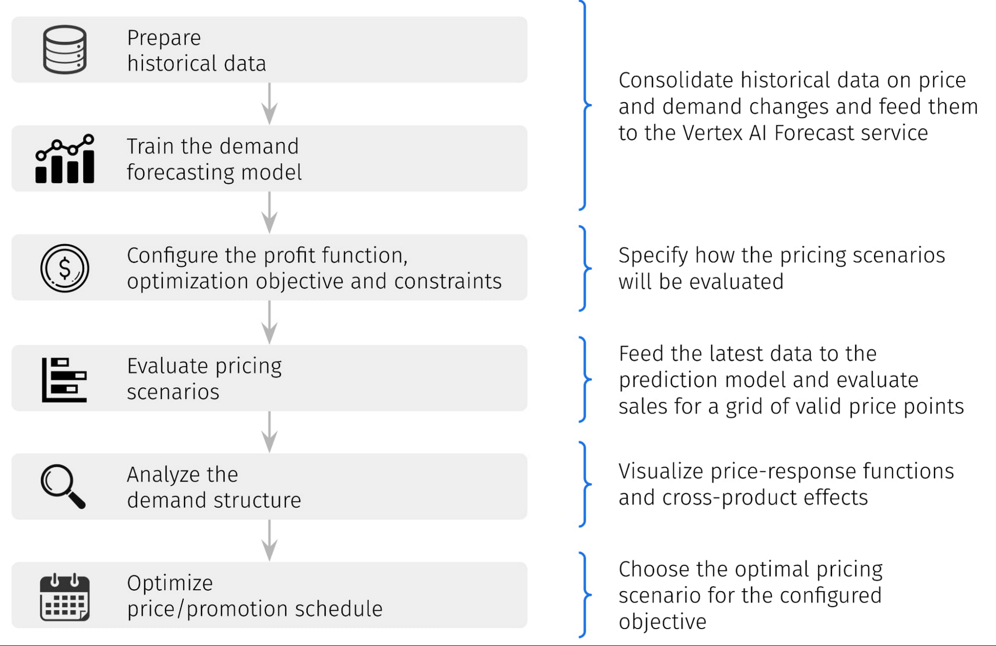
These steps are described in more detail in the next sections, and their reference implementations are represented in more detail in the notebook that accompanies this blog post.

Demand Forecasting Model

Preparing the Training Data

The training data consists of historical data for SKU sales and prices. Vertex AI requires an additional column (“id” in our example) to identify each separate time series (SKUs). In our implementation, the “price” column corresponds to the relative price in respect to the cost:

price = price_dollars / cost_dollars

For example, price of 1.4 means the markup of 40% and a margin of 28.6% (0.4/1.4*100%). There is also a separate column “cost” in monetary units (dollars). Other columns represent various attributes of a particular SKUs, e.g. “category”, “brand”, “gender”, “price_tier”, etc. The usage of attributes allows the model to learn behaviors across SKUs. With these attributes the model can learn to forecast new products' demand, when historical data is not yet available.

Our example data schema can be further extended with external signals such as competitor prices and public events, and also domain-specific attributes such as sales channel qualifiers or store locations. The dataset has to be made available as a CSV file in a GCS bucket or a BigQuery Table.

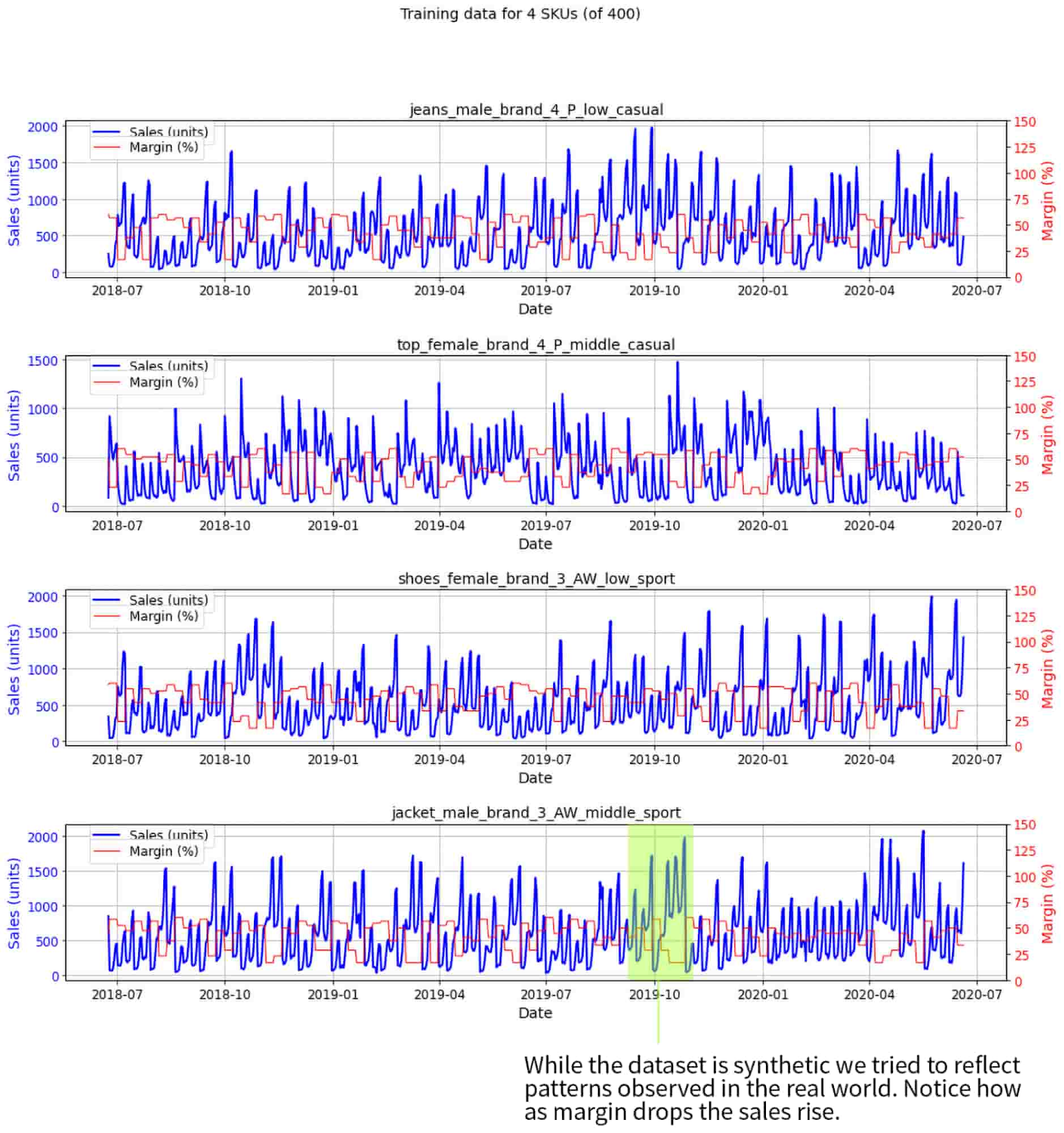
For demonstration purposes, we used a synthetic dataset with seasonal effects modeled after what we observed in real sales datasets. The dataset includes sales-price data for 400 SKUs. The following figure depicts the training data for 4 randomly selected SKUs:

Training the Model

Before training the model you should clearly specify which variables (columns) are covariates, and which are attributes. Covariates can change with time for a single time series (SKU) while attributes are static. In our example, “price” is a covariate, while other variables are attributes. In reality, the number of covariates can be much larger. For example, weather conditions, holidays, competitor prices are all reasonable candidates for your covariates.

Other important model configurations are (1) the length of the context window  and (2) the length of the forecasting horizon. In our example, they are chosen to be 28 and 14 days respectively. Last, you need to choose the loss function and the training budget. In the reference implementation, we use RMSE and 1 hour, respectively.

Basic Price Optimization

Preparing Inputs for Pricing Scenarios Evaluation

We now need to make demand forecasts for multiple price levels. Vertex AI batch prediction service requires submitting a csv file (or a BigQuery table) with the same schema as training data. The file needs to:

• contain historical values for all variables populated for the length of the context window (i.e. 28 days of historical values in our case)

• contain the new dates appended for the duration of the forecast horizon (i.e. 14 days)

• for the dates in the forecast horizon the values of the target variable should be blank

The batch prediction endpoint would return the submitted file where blank values of the target variable are replaced with the model predictions. 

To get predictions for multiple price levels we generated a dataset with M time series for each SKU, where M is the number of different price levels. For each SKU in the resulting file there are

• 1 series of historical values

• 15 series for the forecast horizon values with blank values in the target column (1 series for each of the evaluated price levels).

Evaluating Pricing Scenarios

Now we need to get the forecasts for each of the price levels and pick a price level which maximizes total profit for each SKU. The input file described above needs to be submitted to Vertex Batch Prediction service. After the job is finished (which typically takes 5-10 minutes) the resulting file would be placed in the pre-specified GCS bucket (or a BigQuery Table). 

Here is an example visualization for one of the SKUs in the file. The black line represents the historical context period of 28 days. The colored lines represent the demand for different price levels. Only 5 levels (out of 15) are shown for clarity.

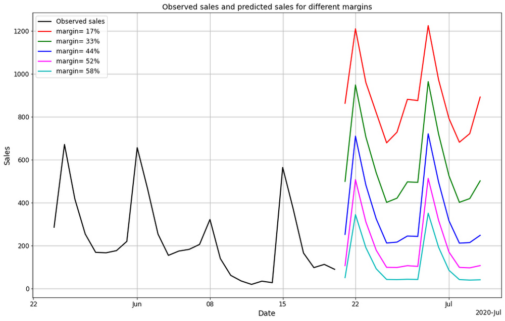
The plots clearly show that the predicted sales have strong dependency on the day of the week and price margin. For example, the red line (lowest margin) has the highest levels of sales and the pattern of sales is different from the blue line (highest margin). Notice how the lines are not just shifting up, but changing shape too - this is a non-linear forecasting model at work.

It is worth noting that, in traditional price analytics, the relationship between price and demand is typically modeled using parametric functions. For example, a “constant elasticity” model is widely used:

demand  = a * price ^ b 

In this model, a and b are the parameters that are inferred from the data. These parameters can be analyzed and compared to baselines to better understand the demand structure. For example, parameter b in the above model is known as the price elasticity of demand, and it characterizes the relative sensitivity of the demand to price changes. The downside of such an approach is that demand response to price changes is often more complicated than the formula suggests.

In our approach we do not make any assumptions about the shape of the price-response function and evaluate it point by point in a non-parametric way. Consequently, the curves for different margin values in the above figure have similar but not identical shapes. We can still assess the traditional metrics such as price elasticity by evaluating the spread between the empirical curves. However, when modeled with ML methods these metrics are allowed to change over time which means we can get more accurate demand forecasts and an overall more flexible and expressive solution.

Analyzing the Demand Structure

Once the demand forecasts are produced, we can visualize the price-response curves and other statistics that help understand the market behavior and demand structure. For example, we can visualize the sales and profit as functions of margin for individual days:

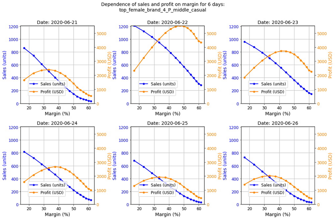
In this particular case, the price-response functions are significantly different for different days of the week, and thus profit-maximizing price points would also be different. In other words, we would need different prices on different days to maximize profits. In this analysis, we used a simple profit function:

profit = demand_units * (unit_price_dollars - unit_cost_dollars)

but in practice the objective function can incorporate additional considerations such as storage or liquidation costs. The starter kit provides the ability to customize the objective function.

Determining the Optimal Price Points

After the sales predictions for different prices margins have been obtained for each of the 15 price points in each day we proceed to evaluate the profit for each point. We used grid search to determine the optimal price for each SKU on each of the dates.

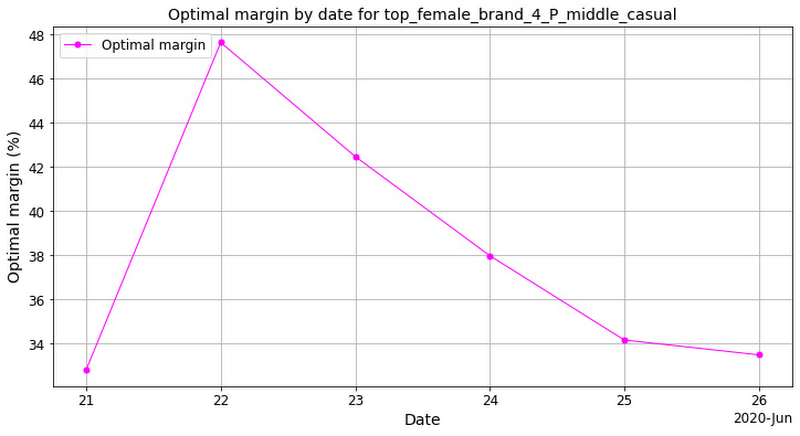
The figure below shows the price level recommendations for one of the SKUs. Different margin values are recommended for different days of the week, which is consistent with the demand structure analysis performed in the previous section.

For simplicity we made a number of assumptions, for example that 

• prices can change daily 

• the only price points available are the 15 points we used and 

• the demand for each SKU is independent.

In real world applications retailers typically update prices weekly, the number of available price points varies per product and various interactions between the SKUs are present (e.g. cannibalization and halo effects). 

The pattern of optimal price levels can be different for different types of products. Some products have constant price-response dependencies - their demand is directly proportional to their price regardless of other factors, like the day of the week. Other products have a price-response function which varies depending on the season, holidays, and other factors. For example, consumers are a lot less sensitive to the price of turkeys during Thanksgiving week.

If we have a large space of valid prices (e.g. from 100 to 500 dollars with a step of one cent) doing individual forecasts for each price point may become impractical. In this case we can interpolate the price-response curve and determine the optimal price using grid search or some other standard maximum search procedure.

Advanced Price Optimization Techniques

The pipeline described above implements the basic price optimization process under a number of simplifying assumptions. In practice, price optimization solutions are more sophisticated and account for many additional constraints, effects, and factors. Here are a few common considerations:

• Cross-product effects. The assumption about independent SKU is not accurate in many real-world environments. SKUs often have cross dependencies because of cannibalization, halo, and other economic effects. This means that the price change for one SKU can impact sales for related SKUs. Both positive interactions (halo effect) and negative interactions (cannibalization) are possible. Inaccurate modeling of such effects can result in suboptimal promotion campaigns and even losses. Joint optimization of prices for multiple interdependent products can also represent a computational challenge. In the next section we provide an example solution to this problem.

• Constrained optimization. In real-world applications, each product is associated with certain supply SLAs. Some products are easily replenishable, some have long lead times or limited supply, and some, especially in the apparel domain, are not replenishable at all. The optimization process often needs to take into account inventory constraints to avoid out-of-stock situations. On the other side are products with limited shelf life, like groceries and many seasonal fashion products. Such products typically need to be sold out entirely by a specific date.

• Historical data availability. Data availability is often a challenge for slow-moving and newly released products. When historical data is limited or not available, custom extrapolation techniques are required to increase the catalog coverage (the percentage of products for which optimization can be performed). The reference implementation partly addresses these issues by enabling transfer learning across SKUs through their product attributes. In practice, more advanced techniques are usually required.

• Scalability. Large apparel retailers often manage hundreds of thousands of SKUs across thousands of locations. The demand patterns can be drastically different across different SKUs and categories. Many retailers use different pricing strategies for different groups of SKUs, for example, to manage key value items (KVIs) differently from slow-moving specialty items. The large number of data sources, model training and data transformation pipelines present unique operational challenges and often require advanced MLOps infrastructure tools and processes. Vertex AI provides a range of MLOps tools to help scale complex ML workloads.

• External factors. The reference pipeline data schema was limited to sales data and few product attributes. In practice, forecasting accuracy can be improved by integrating a broader range of signals such as competitor prices, weather, and public events.

• Dynamic pricing. In highly dynamic environments, such as fashion websites with flash sales, the referenced methodology may no longer work. When sales events are very short-lived, traditional demand forecasting is often too slow or inaccurate. These highly dynamic settings usually require specialized algorithms, often from the domain of reinforcement learning, to dynamically manage prices. 

A thorough discussion of all these advanced scenarios is beyond the scope of this blog post. More content on advanced price and supply chain optimization techniques is available on Grid Dynamics Insights portal.

Optimization with Cross-product Effects

The approach in the starter kit makes the assumption that SKUs are independent. In the presence of cross-product effects such as cannibalization, the demand evaluation model needs to be modified to account not only for the price of a given product, but also for prices of related products. 

One solution is to analyze cross-product dependencies, determine clusters of interdependent products, and create evaluation models which use all individual prices within a cluster. In practice, it can be challenging to evaluate the combinations of individual prices, and more coarse-grained techniques are often used. For example, demand forecasting can be performed using the product’s own price and the average price for all other products within the category or cluster.  

The forecasting model in the starter kit can be customized to evaluate scenarios with multiple interdependent pricing parameters. Such customizations are not included in the reference pipeline. However, if you have already customized your model, the starter kit includes an example of the analysis and evaluation of the cannibalization and halo effects.

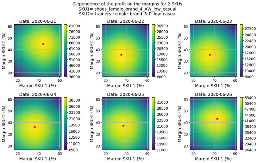
The figure below shows how the total profit for a pair of SKUs can be evaluated for different combinations of the corresponding margins. This evaluation can be performed for individual dates to determine the optimal joint price schedule for two SKUs. The profit value is shown using color coding (yellow is higher). The red point shows the optimal price level, yielding maximum profit.

This evaluation procedure can be combined with grid search to find the optimal price levels for groups of interdependent SKUs.

Business/Real World Use Cases

The reference pipeline assumes a basic, somewhat abstract price optimization scenario. It would require tuning and customization in most real world applications. We discuss these functional aspects of the solution design in a dedicated white paper.     

Here are several common problems and customizations where the reference implementation can be used as a starter kit:

• Promotion optimization. Many retailers have a complex process for promotion calendar management that includes long-term preliminary planning and regular adjustments. The reference pipeline can be used for both long-term planning (e.g. 52 weeks-ahead) and ongoing adjustments on a weekly basis.

• End-of-season clearance. Many apparel retailers practice end-of-season campaigns which require continuous tracking of the sales progress and price adjustments.. Price optimization models need to support the maximization of sell-thru rates, margins, or other metrics under the inventory constraints using markdown adjustments. 

• Inventory turnover optimization. The demand forecasting pipeline can be used not only to support pricing decisions, but also to optimize inventory replenishment decisions based on granular store-level and SKU-level forecasts. The typical objectives include the  maximization of the inventory turnover and improvement of the storage and logistics efficiency.

• Assortment optimization. Demand forecasting at SKU level for individual stores is often used to improve assortment decisions. The forecasting models can be modified to evaluate demand shifts from adding or removing items to the assortment. 

• Back-to-front replenishment. Granular short-term demand forecasting at the store level is sometimes used to improve the movement of inventory from backroom to frontroom. The forecasting solutions are typically integrated with hand-held devices used by store associates to instruct how many units of which items need to be moved.

• Store workforce optimization. Finally, demand forecasts are often used to optimize workforce management decisions and shifts. In practice, retailers often collect the actual store traffic data using in-store sensors, and this data can be used to produce traffic forecasts. A combination of sales and traffic forecasts can be used for workforce optimization.     

Conclusion

GridDynamics prepared the reference pipeline described in this blog post based on numerous price optimization engagements with leading retailers around the world. It illustrates how Vertex AI Forecast can be used to solve price optimization problems in a broad range of industries. It also demonstrates how a large part of the traditional ML workflow can be successfully performed by an AutoML algorithm with minimal human intervention. The colab with the pipeline is a perfect starter kit to accelerate the development of custom price and assortment optimization solutions.