Measuring patent claim breadth using Google Patents Public Datasets

Last fall, we released the Google Patents Public Datasets on BigQuery. These datasets include a collection of publicly accessible, connected database tables that enable empirical analysis of the international patent system. This post is a tutorial on how to use that data, along with Apache Beam, Cloud Dataflow, TensorFlow, and Cloud ML Engine to create a machine learning model to estimate the ‘breadth’ of patent claims. You can find all of the associated code for this post on GitHub. Before diving into how to train that model, let’s first discuss what patent claim breadth is and how we might measure it.

Background

Patents are comprised of a number of sections, including title, abstract, description, and claims. A patents’ claims define the scope of the rights held by the patent owner, and as a result, practitioners focus on evaluating claims. Although patents have multiple claims, practitioners tend to focus on the first claim, because it is typically most illustrative of the patent right. Since manually reading claims is time intensive, considerable effort has been spent to generate "automated" estimations of claim breadth based on scoring the first claim of a patent. In general, these approaches attempt to estimate the “breadth” (or “scope”) of a claim as a proxy for the technology covered by a particular patent.

While there is no official method to measure claim breadth, both patent practitioners and scholars often use word count as a proxy for claim breadth, relying on a simplifying assumption that in general, a longer claim is narrower than a shorter claim. While longer claims may or may not necessarily be narrower, and this post takes no position on the assumption, word count is simple to compute and can be consistently applied to both patent applications and issued patents, leading to wide adoption. In this post, we demonstrate a machine learning (ML) based approach to estimating claim breadth, which has the ability to capture more nuance than a simple word count model. While our approach may be an improvement over simpler methods, it is still imperfect and does not account for any semantic meaning within the text of the claim. This post is not intended to be a recommendation on how to measure claim breadth, but instead we aim to spark academic and corporate interest in using the large amounts of public patent data in BigQuery to further the state of the art in patent research.

Structuring claim breadth as a machine learning problem

In order to use ML to build a model of claim breadth, we need training data. Since no objective measure of claim breadth exists, our approach will rely on two assumptions:

1. Claims in patent applications tend to be broader than claims in issued patents. Typically, the patent examination process results in one or more amendments to the patent claims filed in the initial application that narrow the scope of the final version of the claims in the issued patent. Therefore, the final issued patent generally includes  narrower claims than the initial application.
2. Although this statement does not hold absolutely, claims in patents that are “early” in a technology space tend to be broader than patents that appear later.

By utilizing these two assumptions, we can turn our task of estimating claim breadth into a binary classification problem:

1. Positive Observations (i.e., “1’s”)—The first claim in patent applications which were earlier than other applications and patents in a similar technology space.
2. Negative Observations (i.e., “0’s”)—The first claim in issued patents which were later than other patents in a similar technology space.

After training a model on this classification problem, we can ask the model for the probability that a patent is a positive observation (on a scale from 0-1), and use this as a claim breadth score.

Note that a number of ways to define “early” and “late” exist—and we hope someone will explore that decision in depth, but for this example, we simply assign each patent an early or late label based on where the patent’s priority date falls relative to other patents in a similar technology subspace. To group patents into technology subspaces, we use the Cooperative Patent Classification (CPC) code at the four digit level. Patents with a priority date that falls before the median priority date in its CPC group are deemed “early” and the rest are deemed “late.”  To demonstrate this idea, the following query calculates the median priority year within each CPC group for all Patents filed after 1995 in an E or F classification code:

Challenges posed by our training data

Because of the way we have structured our training data, relying on this early-versus-late distinction, we must be careful to avoid “leaking” any information about time into our model and causing overfitting. For example, if we included an application date feature, the model might learn to use this feature to separate early from late without learning anything about claim breadth. Similarly, we must avoid giving the model the text of the claim, since some words describing new technologies only appear in later claims. As a result, rather than utilizing more common text-embedding approaches, our model relies on features that are unique to patents, which we will discuss in more detail below.

Preparing training data using Cloud Dataflow

In order to train a model which generalizes well, we’ll want to use a large set of training data. Luckily, we can easily access millions of examples using the Google Patents Public Datasets on BigQuery. We’ll also need to do some preprocessing to this data before training our ML model, including feature engineering and splitting into train and test sets. Since we have a relatively large dataset, we’ll use Apache Beam running on Google Cloud Dataflow to preprocess our data in parallel in a matter of minutes. The pipeline performs the high level steps below, and the full code is available here:

1. Run a query against the patents.publications table to retrieve all US patents and applications in a specified set of CPC codes with priority dates later than a user specified year. The query results include the full text of the claims and other metadata we need for training our model.
2. Extract the first claim from the full text of the document’s claims.
3. Create features from the text of the first claim.
4. Split data into train/test/evaluation sets and write to TFRecords files on Google Cloud Storage.

Prerequisites

Before running the examples below, you may need to do some initial setup. For a detailed description, please check out the prerequisites section of our README on GitHub.

Running the preprocessing pipeline

To run the preprocessing code and generate training and evaluation data, simply run the preprocessing.py file using the DataflowRunner:

This will launch a job on Google Cloud Dataflow, and you can monitor the job from the web UI. The web UI should show your job’s graph, alongside useful counters and metrics from job execution. When the job completes (~20mins depending on the number of workers), your graph should look like this:

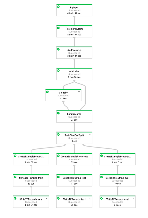
In the next section, we’ll use the output of this pipeline to train a claim breadth model, but first we will briefly discuss how the pipeline works. To see the full code, view preprocess.py.

Pipeline input from BigQuery

The query input to this step is constructed using command line options that allow the user to control the priority dates and CPC codes included in our data. This is useful for building models tailored to a specific time range or technology area. For example, to get training data for recently issued patents in the E and F class codes we would run the following query:

This query retrieves the full text of the patents’ claims, priority year, and the publication number from Google Patents Public Data along with an array containing publication year quantiles. We’ll use this array later in the pipeline for adding an inferred class label.

Extracting the first claim

As mentioned above, patents often have multiple claims, however practitioners tend to focus on the first claim. For this reason, our framework will require an algorithmic way to keep only the text of the first claim. Fortunately, most US patents tend to follow a standard structure like:

What is claimed is:

1. A widget, having… with
Some feature;
Another feature;
…
And a final feature;

2. The widget in claim 1 with…
….

This structure enables clean extraction of the first claim with simple pattern matching that works most of the time. In our pipeline, this is done by passing our PCollection through a Beam DoFn which handles this pattern matching logic and counts failures so we know when things aren’t going well.

Feature engineering

Now that we have our first claim, we can add any features that might be relevant for our ML classification task of separating broad patents from narrow patents. As discussed in the introduction, we must avoid using features which capture semantic meaning, since these could be used by the model to learn to separate early patents from late patents without learning anything about claim breadth. Therefore, we’ll focus on capturing features in two categories:

1. Features related to claim structure and syntactic complexity.

2. Features which count the appearance of words and phrases that tend to narrow or broaden a patent’s claims.

One of the simplest ways to capture complexity is to count semicolons, which are used to separate elements in a claim. Additionally, we can count words and phrases that tend to have a specific impact on patent claims. Some examples are words like “exclude”, “include”, “without”, “with”, etc.. The list of potential features could go on and this post isn’t aimed at describing the ideal feature set. Instead, we aim to give readers a framework for approaching experimentation. Please feel free to fork our repository and experiment with your own features. A few examples are below:

• How often do excluding phrases like “or”, “not”, “exclusive”, “only”, “without” appear?

• How often do counting words like “second” or “third” appear?

• How often does a digit or decimal appear?

• How many elements (separated by semicolons) are in the claim?

To handle most of our feature generation in our pipeline, we can rely heavily on regular expressions (regex). For each feature, we simply define a regex that captures a word or group of words and add it to a set of patterns, then hand this off to a Beam DoFn, which adds the counts to our PCollection. A simplified example is shown below:

Splitting into train, evaluation and test sets

Creating TensorFlow examples and saving to TFRecord files

In the next section, we’ll be working with the TensorFlow Datasets API which works nicely with TF Records format, so in this last step, we’ll convert our Beam PCollection from a collection of python dictionaries into TensorFlow Examples and write to TFRecords Files:

We do this for each of the three splits from our last step and since beams WriteToTFRecord shards by default end up with 3 sets of TFRecord files:

With our training data set up, we’re ready to train our model.

Training our model on Cloud ML Engine

Now that we have our data prepped, we can train our claim breadth model. For this example, we’ll be training a deep neural network on Cloud ML. As a starting point, we’ll train a DNNClassifier, which is one of the premade estimators included with Tensorflow. Premade estimators make training models on GCP extremely easy and handle many of the challenging parts of doing scalable machine learning. If you’re already familiar with TensorFlow, you could easily substitute our premade estimator with your own custom estimator.

You could train this model locally using the same estimator, but for demonstration purposes, we’re going to walk through the steps to train your model on Google’s ML Engine. ML Engine has two main benefits. First, you can write code once, then easily switch between training locally on your own hardware, or scale up to multiple GPUs with a simple command line flag. Second, you can easily run a hyperparameter tuning experiment without modifying your training code at all.

The Cloud ML Engine documentation has great information on how to package your training application, so we won’t go into too many details here. For a demo of the main concepts, have a look at this excellent tutorial which walks step by step through the main concepts we use here.

At a high level we have two main files:

• Model.py: Which handles the following:

• Defines an input function, which instructs TensorFlow what to do with the TFRecords files we created in the preprocessing step.

• Defines a model constructor function, which configures the DNNClassifier with the appropriate parameters.

• Defines a serving function, which allows us to reuse the trained model for inference later. More on this in the next section.

• Task.py: Which handles the following:

• Parses our command line flags and passes them to the input and model functions.

• Starts a training and evaluation loop using estimator.train_and_evaluate

Embedding CPC codes

Before training our model, we need to handle one key prerequisite,setting up a vocabulary file for an embedding column in the model. Our training data includes a string feature ‘CPC4’ which is the patent’s CPC code at the 4 digit level. Including this feature is critical to having a useful model because it allows the model to learn something about how a patent’s technology space changes the impact of our features on claim breadth. Without this feature, our model would have to find one mapping between our input features and an output label regardless of technology area—which is not ideal, because claims can vary widely across technologies.

Because neural networks expect numeric inputs, we need to convert this string variable into some numeric format. The two most common approaches here are indicator columns and embedding columns. The TensorFlow documentation has a great overview of both approaches.

For this model, we choose to use an embedding column which requires a “vocab list.”  Each CPC code on our list will get an embedding of its own and any CPC not on our list will be lumped into an “UNKNOWN” category. One approach would be to let the model have a list of all possible CPC codes, but this is not ideal since some CPC codes may be very rare in the training data and might cause the model to overfit. For this reason, we keep only the CPC codes with a large number of examples in our training data.

To build this list, we run a query against the Patents Public Data on BigQuery and write a text file to Cloud Storage:

An example query is included in our repository, but which CPC codes to keep and which to exclude is a design decision that should be explored by the end user of this model.

Launch the training job

To launch a training job in Cloud ML Engine, we’ll first need to set up a few variables to pass to our training command. The commands below assume you already created the training and evaluation files by running the preprocessing step above.

With those argument variables set, we can launch a training job in the cloud:

You can monitor training progress several ways: by streaming logs to your terminal, viewing logs on the web, or for a more interactive view, you can also follow training progress by running TensorBoard. Because we are training with estimator.train_and_evaluate and using a premade estimator, TensorFlow will automatically write some useful metrics to the location defined above as $GCS_JOB_DIR. To run TensorBoard run the following command:

tensorboard --logdir=$GCS_JOB_DIR

This should open a new browser window and as training progresses, you’ll see various metrics updating. Some metrics, like loss, will update with each step during training, while others, like AUC, will only update each time an evaluation is run against our held out evaluation data. To control the frequency of evaluation, take a look at the --eval-secs argument in task.py.

As training progresses, we see our loss curve dropping, indicating that our model is learning:

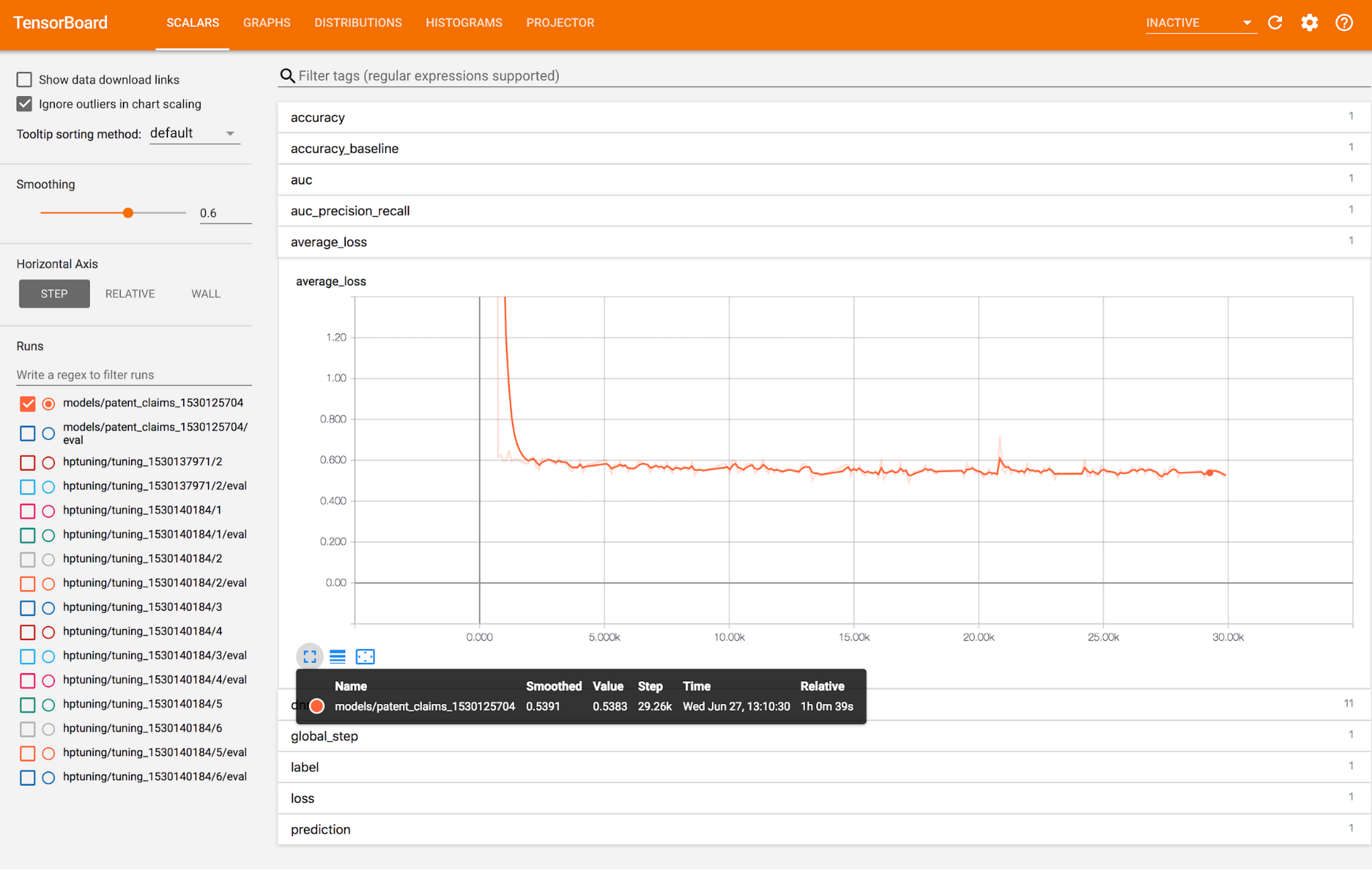
In the run above, we’ve set the model to train for 30,000 steps with a batch size of 512 per step, which means the model will run roughly 19 epochs over the full training set produced in the preprocessing step. For this particular run, the model reached an evaluation AUC of 0.802.

Exporting a saved model

If you want to use your trained model for inference, you’ll need to export a final model at the end of training. We handle this in model.py, where we define a JSON serving function that tells TensorFlow how to map a JSON input to the model’s input tensors. When the model finishes training, a set of SavedModel files will be saved to an `export` folder inside the bucket you defined in $GCS_JOB_DIR. We’ll use this exported model in the final steps later when we move on to using Cloud ML’s prediction API for inference in the next step.

Hyperparameter tuning

Running batch inference

Now that we’ve trained our model, we’d like to score a large set of US Patents to enable us to use claim breadth alongside all the other great data in the Google Patents Public Datasets. One option would be to load our saved model in memory and step through all US patents in serial, but this would take a long time, so instead we’ll use Google Cloud Dataflow along with ML Engine to do batch inference and write our predictions out to BigQuery.

The first step will be getting our trained model set up on ML Engine for online and batch prediction. There are several ways to do this, which are covered in this documentation page. We’ll be using the gcloud SDK to handle it from the command line.

The first step is to create a “model” and a “model version” which is essentially mapping a set of SavedModel files on Cloud Storage to a Cloud ML prediction endpoint:

With the model loaded into ML Engine, we can now use it to make online predictions through a RESTful API. The Cloud Dataflow job we will run in the next step will use this API to score each patent during inference.

Before you run the Cloud Dataflow job for batch inference, you’ll need to decide which patents to run inference against. One option is to just score every example we created in the training step, but since our training examples only include a fraction of the US publications, we will want to rerun the preprocessing step to get all US publications in a set of CPC codes published since 1995. To do this, we’ll simply rerun our preprocess.py file with two additional flags: --pipeline_mode=inference and --query_keep_pct=1.0

Depending on the number of workers you select, this should take about 20 minutes to run. Once it’s complete you’ll be ready to run the next step, which is a second Apache Beam pipeline that handles three main tasks:

1. Reading the TFRecords files you wrote in the last step.

2. Sending a POST request to our ML Engine model’s prediction endpoint to retrieve a score.

3. Writing each score to a table in your BigQuery project.

We won’t go into too many details on the pipeline, but take a look at the full code in batch_inference.py. The core part of this pipeline is in the DoFn RunInference:

This will kick off a batch_inference job which could take many hours depending on the size of your input data. You can speed up the process by adding more workers with the --num_workers command line flag, but keep on eye on your prediction API quota, as more workers will increase the number of requests being made to your prediction API.

Analyze in BigQuery

Once the job finishes, you’ll have a new table in your BigQuery project based on the flags specified in the command above.

With this new table, you can now connect back to the patents public data and run queries joining your claim breadth table with many other tables. Here’s one example to get you started which calculates average breadth by both art unit and by priority year:

Conclusion