Coastal classifiers: using AutoML Vision to assess and track environmental change

Tracking changes in the coastline and its appearance is an effective means for many scientists to monitor both conservation efforts and the effects of climate change. That’s why the Harte Research Institute at TAMUCC (Texas A&M University - Corpus Christi) decided to use Google Cloud’s AutoML Vision classifiers to identify attributes in large data sets of coastline imagery, in this case, of the coastline along the Gulf of Mexico. This post will describe how AutoML’s UI helped TAMUCC’s researchers improve their model’s accuracy, by making it much easier to build custom image classification models on their own image data. Of course not every organization wants to analyze and classify aerial photography, but the techniques discussed in this post have much wider applications, for example industrial quality control and even endangered species detection. Perhaps your business has a use case that can benefit from AutoML Vision’s custom image classification capabilities.

The research problem: classification of shoreline imagery

The researchers at the Harte Research Institute set out to identify the types of shorelines within aerial imagery of the coast, in order to accurately predict the Environmental Sensitivity Index (ESI) of shorelines displayed in the images, which indicate how sensitive a section of shoreline would be to an oil spill.   

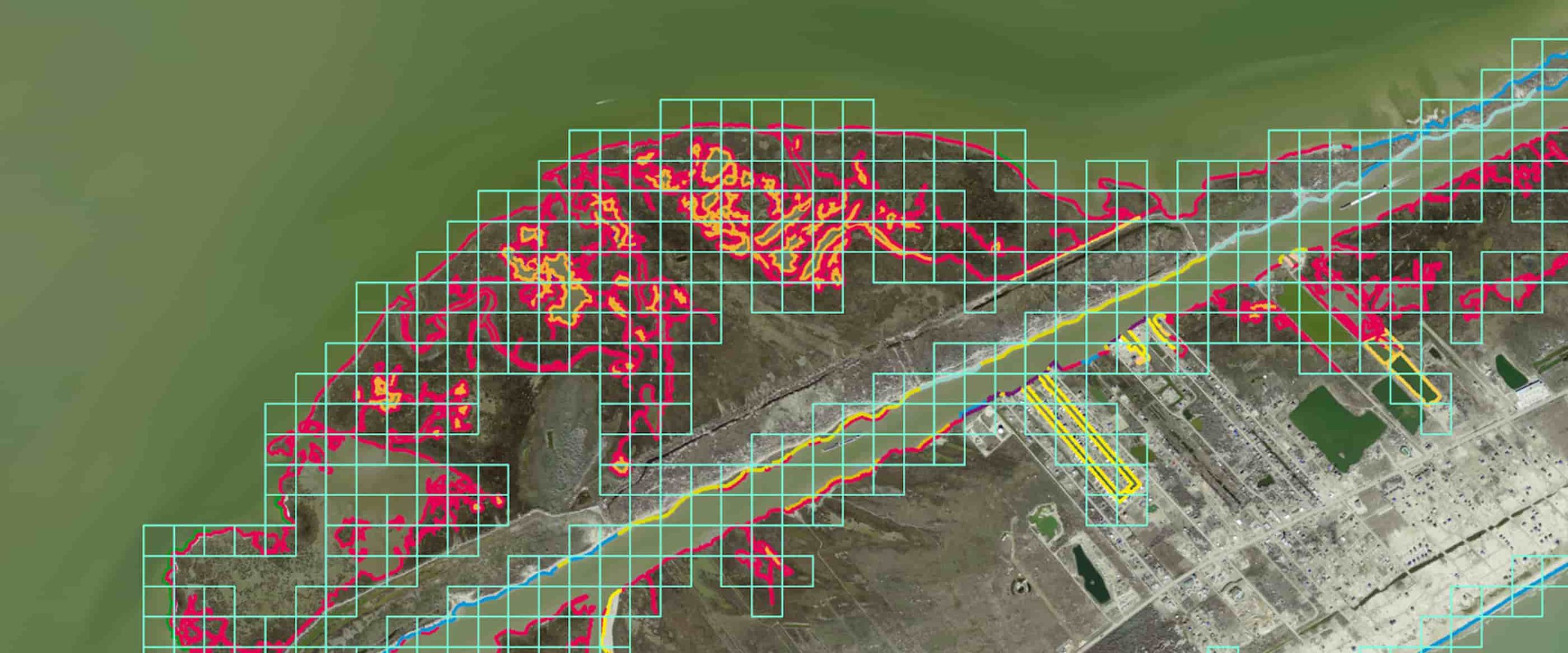
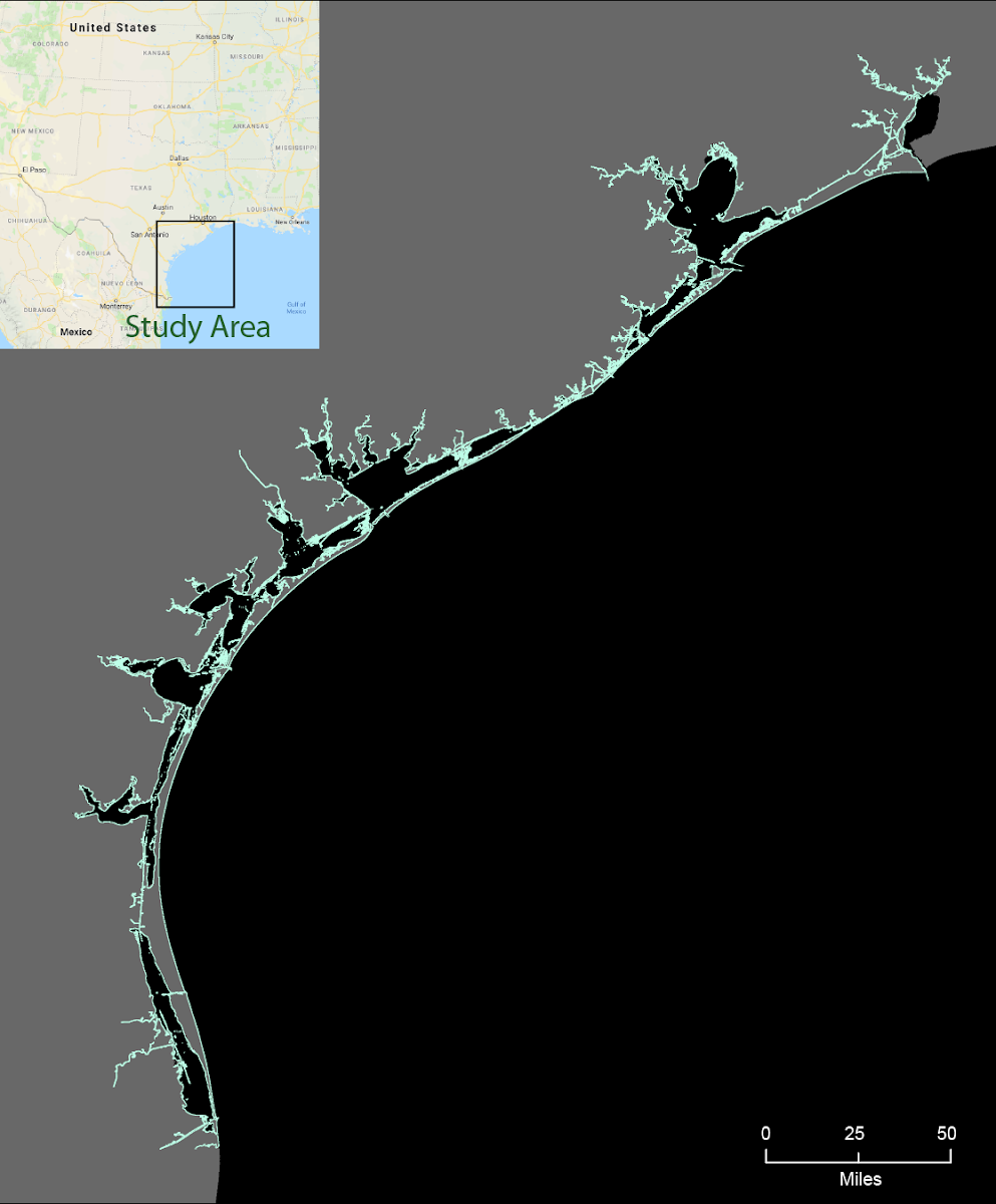
Anthony Reisinger and his colleagues at the Harte developed an Environmental Sensitivity Index map of shorelines that may be impacted by oil spills for the State (government) of Texas. During this process, the team looked at oblique aerial photos and orthophotos similar to what one might find on Google Maps, and manually traced out shorelines for the entire length (8950 miles) of the Texas coast (see below). After the team traced the shoreline, they then coded it with ESI values that indicate how sensitive the shoreline is to oil. These values were previously standardized by experts who had spent many years in the field and scrutinizing coastal images.

After an oil spill, the State of Texas uses these ESI shoreline classifications to send out field crews to highly sensitive environments near the oil spill. The State then isolates sensitive habitats with floating booms (barriers that float on water and extend below the surface) to minimize the oil's impact on the environment and the animals that live there.

As you might imagine, the process of learning how to identify the different types of environment classifications and how sensitive these shorelines are to oil spills takes years of first-hand experience, especially when imagery is only available at different scales and resolutions. Some of the team’s research over the years has utilized machine learning, so the researchers decided to see if their expert knowledge could be transferred over to a machine and automate the identification of the different types of ESI shorelines within the images and among the different types of imagery used.  

Coastal environments can rapidly change due to natural processes as well as coastal development, thus, the state needs to update its ESI shoreline assessments periodically. At the moment, the team plans to update the ESI shoreline data set for the entire Gulf Coast that lies within the State of Texas. During this process, new oblique imagery will be acquired to help identify the shorelines sensitivity to oil spills. With AutoML Vision, the team takes newly-acquired oblique imagery and predicts the ESI values in the shoreline photos, thereby classifying (or coding) the new shoreline file we create.

Imagery types

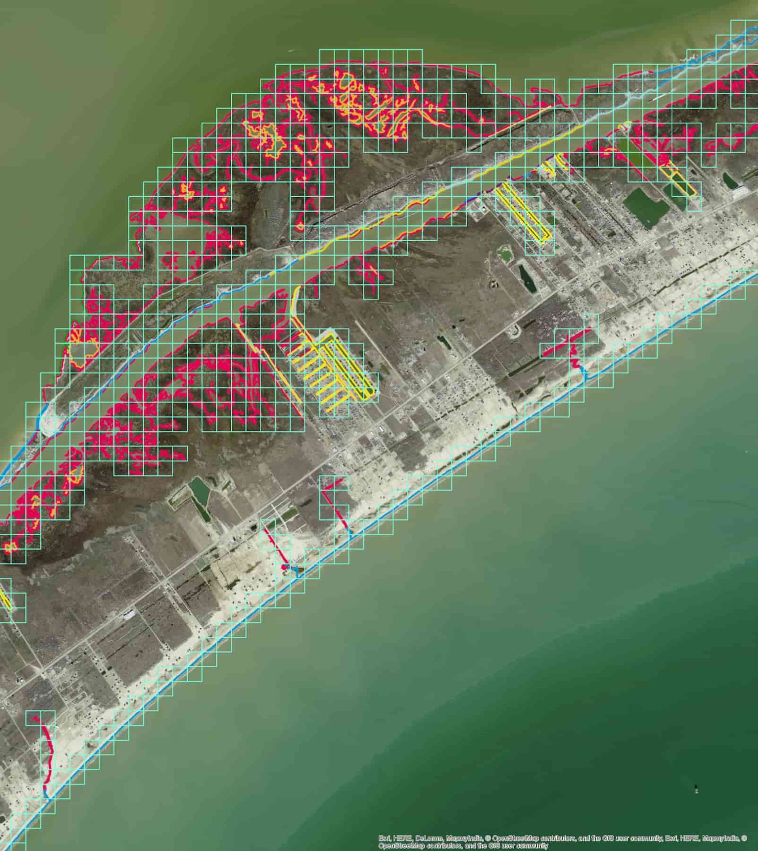
The team experimented with two different types of aerial shoreline images: oblique and orthorectified. For orthorectified aerial photos, a grid was overlaid on the imagery and ESI shorelines, and both were extracted for each grid cell and joined together. For the oblique shoreline photos, the team experimented with applying both single labels and multiple labels (also known as multi-class detection). Details of this latter approach are mentioned later in this post.

But to begin, let’s take a look at the results on the oblique image set. Early experiments comparing precision and recall metrics of AutoML models using orthorectified aerial photos of different pixel resolutions and acquisition dates were compared to AutoML models of oblique photos. Interestingly, the team found that prediction accuracy using oblique imagery models was higher than that for orthorectified imagery models. The oblique imagery models' higher performance is likely due to larger geographic coverage of the oblique imagery, and the inclusion of vertical information in these images.

Cloud Vision’s limitations for our use case

A little testing confirmed that the out-of-the-box Cloud Vision API won’t help with this task: Cloud Vision can identify many image categories, but, unsurprisingly, the results proved too general for the team’s purposes.

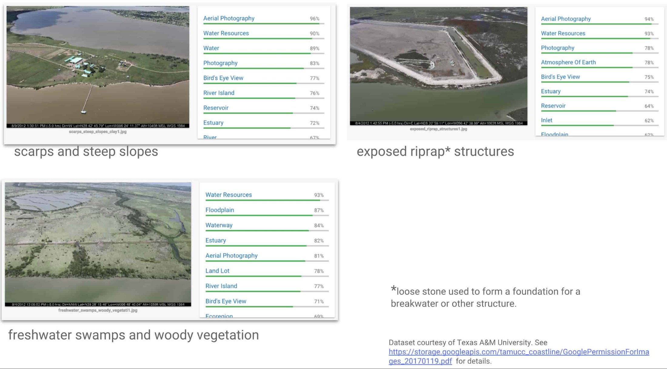
The team then decided that the shoreline images dataset is perfect for use with AutoML Vision, which let the team build their own domain-specific classifier.

Cloud AutoML Vision provides added flexibility

Cloud AutoML allows developers with limited machine learning expertise to train high-quality models specific to their data and business needs, by leveraging Google’s state-of-the-art transfer learning and Neural Architecture Search technology. Google’s suite of AutoML products currently includes Natural Language and Translate as well as Vision, all currently in beta.

By using AutoML Vision, the team was able to train custom image classification models with only a labeled dataset of images. AutoML does all the rest for you: it trains advanced models using your data, lets you inspect your data and analyze the results via an intuitive UI, and provides an API for scalable serving.

The first AutoML experiment: single-labeled images

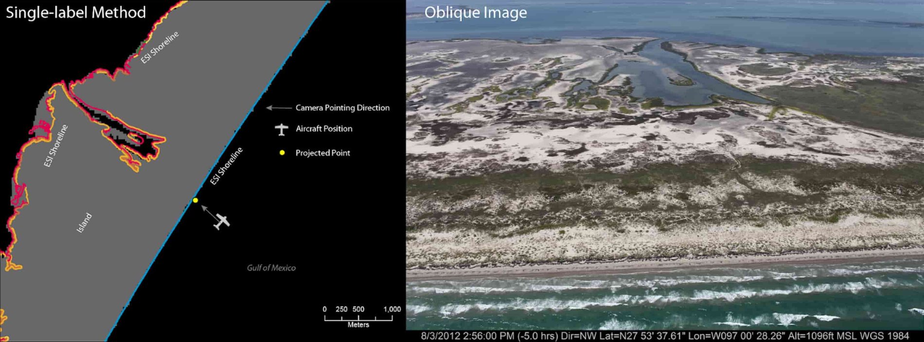
The team first experimented with a single-label version of the oblique image set, in which the label referred to a single primary shoreline type included in the image. The quality of this model was passable, but not as accurate as the team had hoped. To generate the image labels, the direction of the camera and aircraft position were used to project a point to the closest shoreline, and each image was assigned a label based on both the camera’s heading and the proximity of the shoreline to the plane’s position.

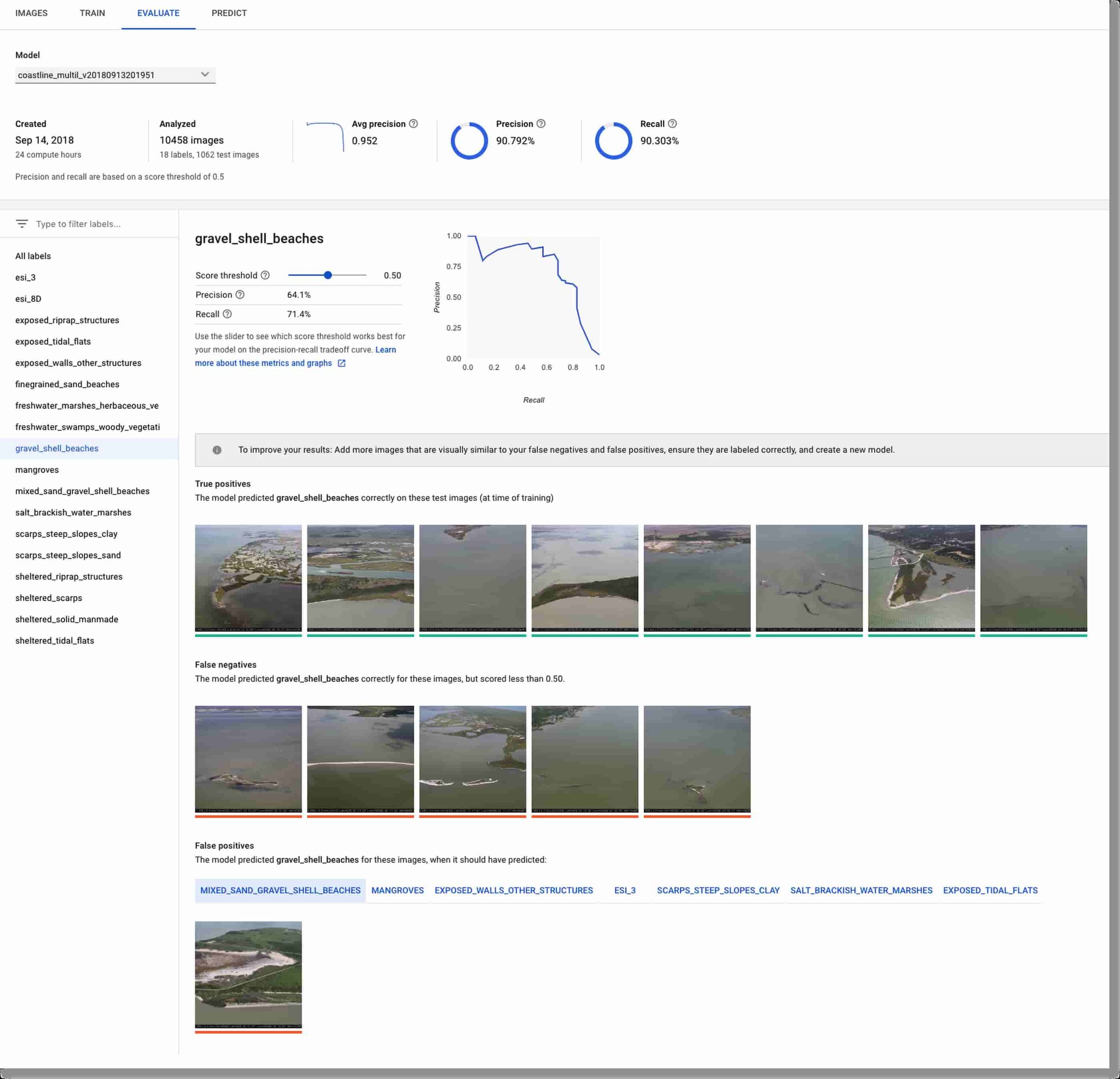
The AutoML UI allows easy visual inspection of your model’s training process and evaluation results, under the Evaluate tab. You can look at the metrics for all images, or focus on the results for a given label, including its true positives, false positives, and false negatives. Thumbnail renderings of the images allow you to quickly scan each category.

From inspection of the false positives, the team was able to determine that this first model often predicted coastline types that were actually present in the image, but did not match the single label. Below, you can see one example, in which the given coastline label was salt_brackish_water_marshes, but the model predicted gravel_shell_beaches with higher probability. In fact, the image does show gravel shell beaches as well as marshes.

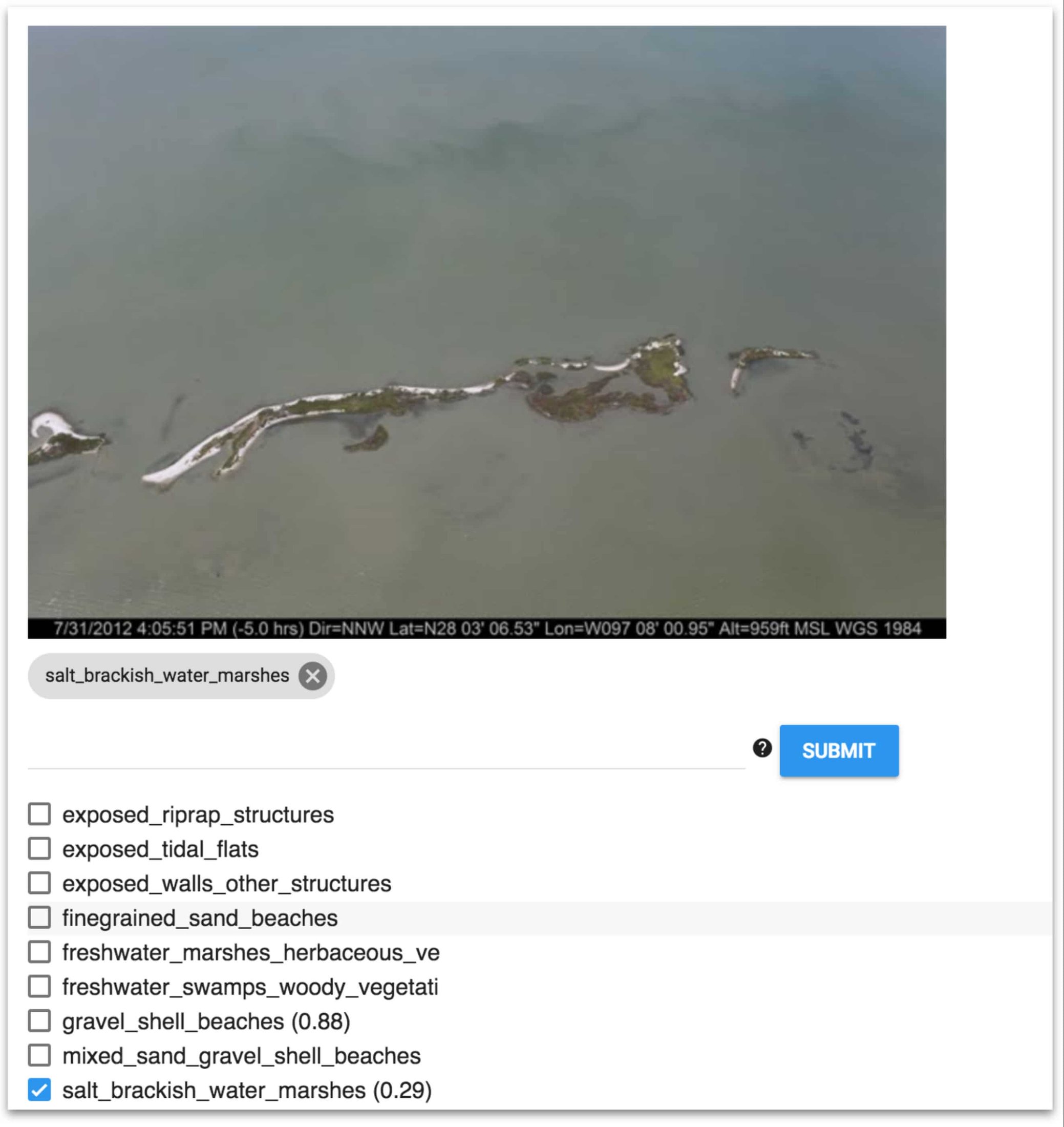
After examining these evaluation results, the team concluded that this data would be a better fit for multi-label classification, in which a given image could be labeled as containing more than one type of shoreline. (Similarly, you might want to apply multiple classes to your training data as well, depending on your use case.)

The second AutoML experiment: multi-labeled images

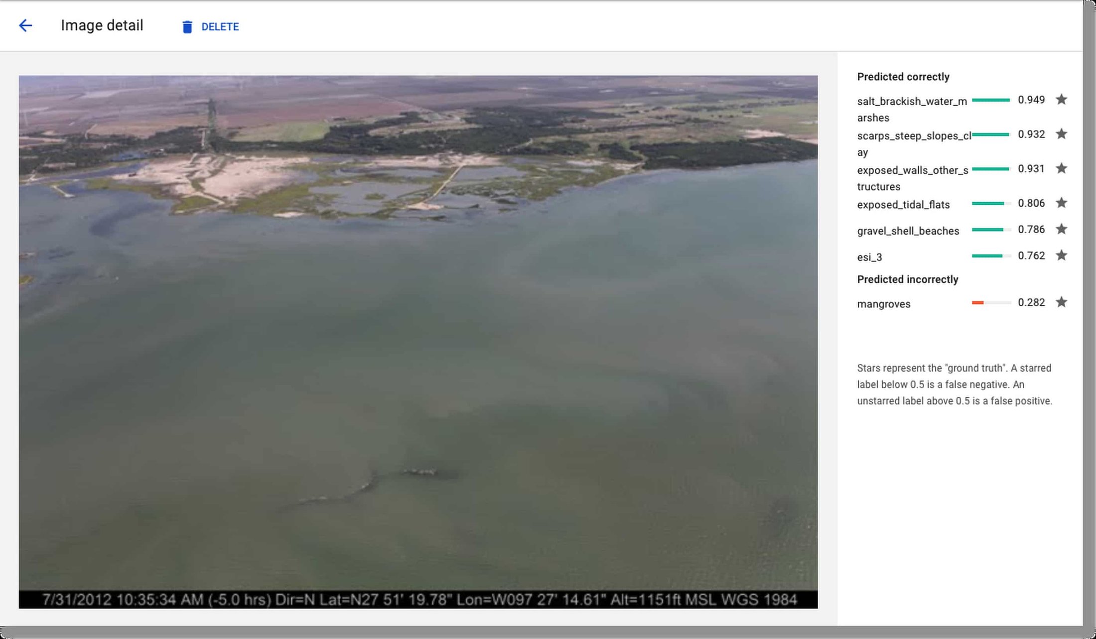
AutoML supports multi-labeled datasets, and enables you to train and use such models. With this capability in mind, the team soon discovered it was possible to generate such a dataset from the original source images, and then ran a second set of experiments using the same images, but tagged with multiple labels per image, where possible. This dataset resulted in significantly more accurate models than those built using the single-label dataset.

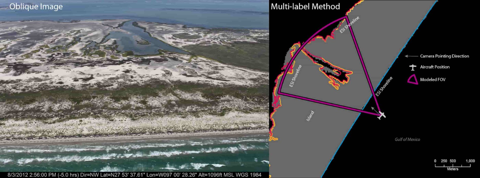
The following image is representative of how the multi-labeling helped: its labels include both gravel_shell_beaches and salt_brackish_water_marshes, and it correctly predicts both.

Viewing evaluation results and metrics

AutoML’s user interface (UI) makes it easy to view evaluation results and metrics. In addition to overall metrics, you can view how well the model performed with each label, including display of representative true positives, false positives, and false negatives. A slider lets you adjust the score threshold for classification—for all labels or for just a single label—and then observe how the precision-recall tradeoff curve changes in response.

Often, classification accuracy is higher for some labels than others, especially if your dataset includes some bias. This information can be useful in determining whether you might increase model accuracy by sourcing additional images for some of your labels, then further training (or retraining) them.

Comparing models built using the same dataset

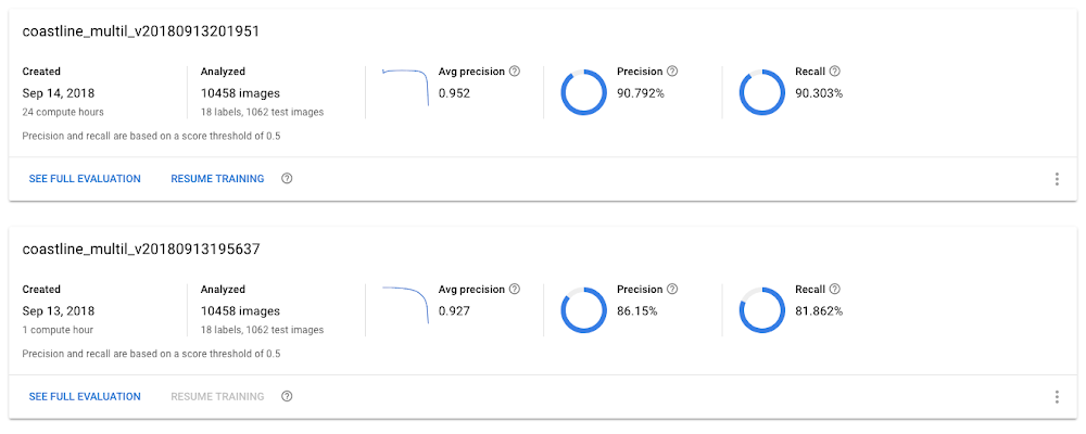
AutoML Vision allows you to indicate how much (initial¹) compute time to devote to creating a model. As part of the team’s experimentation, it also compared two models, the first created using one hour of compute time, and the other using 24 hours. As expected, the latter model was significantly more accurate than the former. (This was the case for the single-label dataset as well.)

Using your models for prediction

AutoML Vision makes it easy for you to use your trained models for prediction. You can use the Predict tab in the UI to see visually how a model is doing on a few images. You can use the ‘export data’ feature in the top navigation bar to see which of your images were in which data set (training, validation, or test) to avoid using training images.

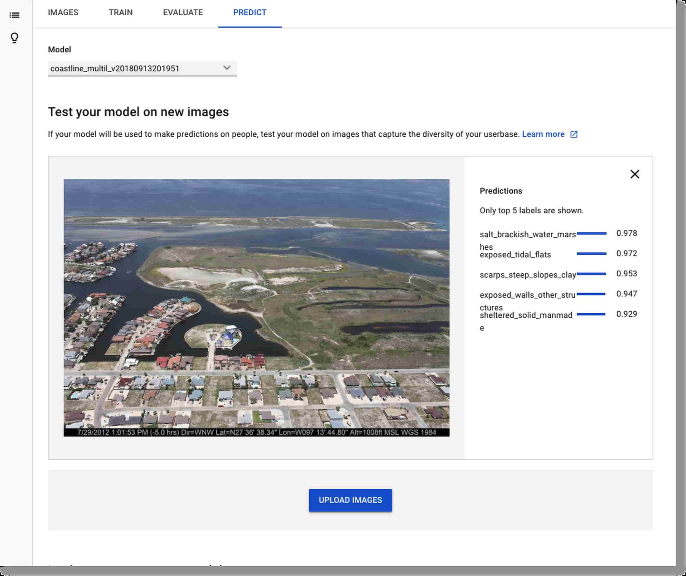
Then, you can access your model via its REST API for scalable serving, either programmatically or from the command line. The Predict tab in the AutoML UI includes examples of how to do this.

What’s next

We hope this helps demonstrate how Cloud AutoML Vision can be used to accurately classify different types of shorelines in aerial images. We plan to create an updated version of the ESI shoreline dataset in the future and use the AutoML model to predict shoreline types on newly acquired oblique photography and orthorectified imagery. Use of AutoML will allow non-experts the ability to assign ESI values to these shorelines we create.

Try it yourself

The datasets we used in these experiments are courtesy of the Harte Research Institute at the Texas A&M University - Corpus Christi. You can use these datasets yourself. See this README for more information, and see this documentation page for permission details. Of course you can use the same techniques to classify other types of geographical or geological features, or even entirely unrelated image categories. AutoML Vision lets you extend and retrain the models that back the Cloud Vision API with additional classes, on data from your organization’s use case.

Acknowledgements

Thanks to Philippe Tissot, Associate Director, Conrad Blucher Institute for Surveying and Science, Texas A&M University - Corpus Christi; James Gibeaut, Endowed Chair for Coastal and Marine Geospatial Sciences, Harte Research Institute, Texas A&M University - Corpus Christi; and Valliappa Lakshmanan, Tech Lead, Google Big Data and Machine Learning Professional Services, for their contributions to this work.

_{1. For options other than the default ‘1 hour’ of compute time, model training can be resumed later if desired. If you like, you can add additional images to the dataset before resumption.}