AI in motion: designing a simple system to see, understand, and react in the real world (Part II)
Noah Negrey
Cloud Developer Programs Engineer
Yu-Han Liu
Developer Programs Engineer, Google Cloud AI
In the first of three posts, we described why we chose to build an AI-powered system that can see, understand, and react to the world around us. We shared our design goals, architectural decisions, gameplay plans, and the process we planned to use. In this post, we will walk through how we gathered data, then how we selected and trained our models.
Gathering and preparing data
One of the first practical steps in any machine learning project involves gathering and preparing the data. In our case we didn’t have a treasure trove of existing labeled data that we could use to train our model, which meant for this project, we needed to create the dataset. There are many ways you might create a dataset, and we considered the brute force approach of taking many photographs individually by hand, or exportingtaking frames fromoff videos, but that would have required a lot of time to label the resulting images with bounding boxes. A better approach for an image-based “seeing” project like this was to automate a process to randomly generate that data using cropped images.
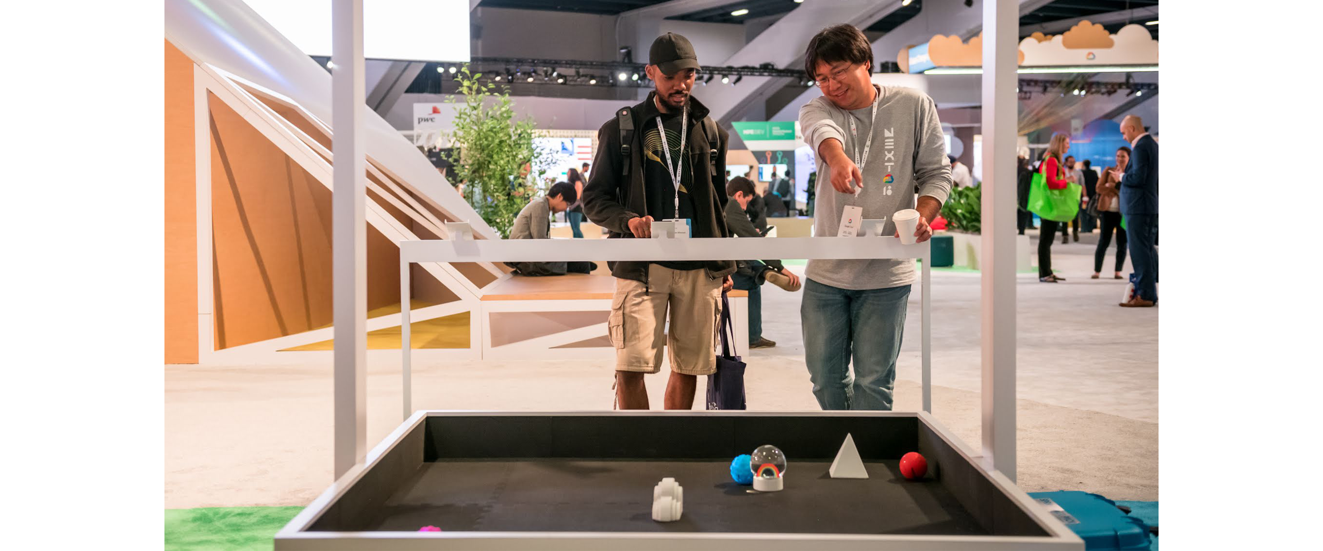
We started with a simple base image of the game arena (Figure 1). The floor, or background, was a black mat typically used in gyms and brown wood pieces which acted as the walls to the arena. Next, we created a simple cropped image of a Sphero robot (Figure 2). These base images would be used to create an automated process to randomly place robots in arena images, and those generated arena images would become our dataset.
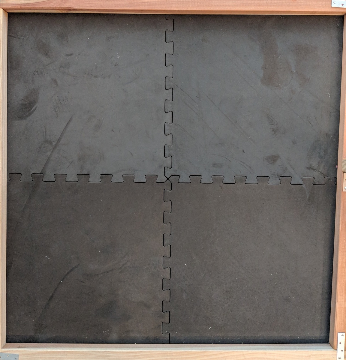

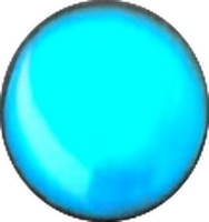

We initially started with two base images and ten different images of the Sphero robot. As the project grew we added more images to add volume and variety to out initial dataset.
We started simple with our generated images, creating a single robot on the base arena image. Later, as we increased complexity by adding objects and more robots, our generated training images looked more like the eventual games. In more advanced images, the floor mats were textured differently, there were multiple robot balls, each robot had a different color cover on it, and there were several additional objects and obstacles of different shapes (Figure 3).
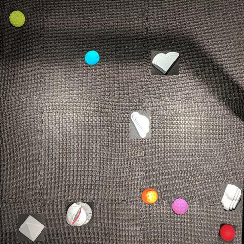

Over the course of the project we photographed and cropped many images to use in our dataset. More than 16,000 images were automatically and randomly generated for training and test images. We used the open-source Python imaging library, Pillow, to do this generation.
Our approach followed Sara Robinson’s Taylor Swift Detector blog guide with one exception: we didn’t manually label our images because we generated our own dataset from scratch.
We wrote a python script (overlay.py) that used Pillow to randomly place our cropped images over our base images. We then stored the location and type for each object in our image to use as our labels. The information we stored for each overlaid image was the coordinates of the image, and we used a bounding box with a normalized coordinate system (left, top, right, bottom), and the type of the image (1 = blue Sphero, 2 = green Sphero, …)
So for one image the labeled information might look like the following:


For additional objects that entry would extend in the same pattern, four coordinates and one label indicating the type of object.
After we generated our dataset and label information, we followed Sara Robinson’s guide on converting that information into a format that TensorFlow accepts, a TFRecord. We took Sara’s script for this conversion and modified it and created our own script to convert the information to a TFRecord for our dataset.
Generating the data required three steps:
Generate a dataset with labels from cropped images—we started with a small number of images, and expanded our dataset as we retrained our model.
Convert the dataset into a TFRecord to be used by TensorFlow.
Upload the TFRecord files to Cloud Storage for use by the Object Detection Model training pipeline.
Choosing a model
Once we had usable data, we focused on selecting the right machine learning models for object detection (Object Detection Model) and ball direction driver (Commander Model). As stated earlier, our Object Detection Model would ‘see’ the arena, robots, and objects, while our Commander Model would ‘react’ in near real-time, with predictions for the optimal robot path. Both models had to be small so they could be on a mobile device.
Object detection
For object detection, we started with a sample application provided by TensorFlow. We used the application as the basis of our app, because it handled several core challenges of seeing the robots: getting access to the camera, pulling images to be for use in object detection, and using TensorFlow on Android. We had to modify the inputs and outputs of the TensorFlow library, and then drop our model into the on device app.
These resources helped us get started with TensorFlow and Android:
Taking our cue from these blog posts, we decided to use the TensorFlow Research team’s publicly posted TensorFlow Object Detection API. This meant we could download one of the checkpoints and modify some of the config files to get our model ready for training.
TensorFlow open source resources:

Modifying the config files for Object Detection
We again referred to Sara Robinson’s Taylor Swift Detector blog on adding the MobileNet checkpoints for transfer learning. The guide provides a great explanation of how to do this, and the short version is that we went through the prepared config file and adjusted the PATH_TO_BE_CONFIGURED placeholders with the location of our data stored in Cloud Storage. To train a quantized model we added the quantization graph rewriter to our pipeline config:Commander model
Our Commander Model uses information from the Object Detection Model to make decisions on where the AI robots should go. Using information about where objects were located, the Commander Model delivers its best prediction of which direction the robot ball should move to win the game. The Commander Model runs each time the Object Detection Model delivers a new image and the model delivers directions for two scenarios: when the robot is a chaser and when the robot is a runner. The chaser tries to tag the other Sphero robots while the runner tries to avoid being tagged - and sometimes tries to unfreeze other robots. The Commander Model also creates paths that help the robot avoid becoming stuck by avoiding the obstacles.
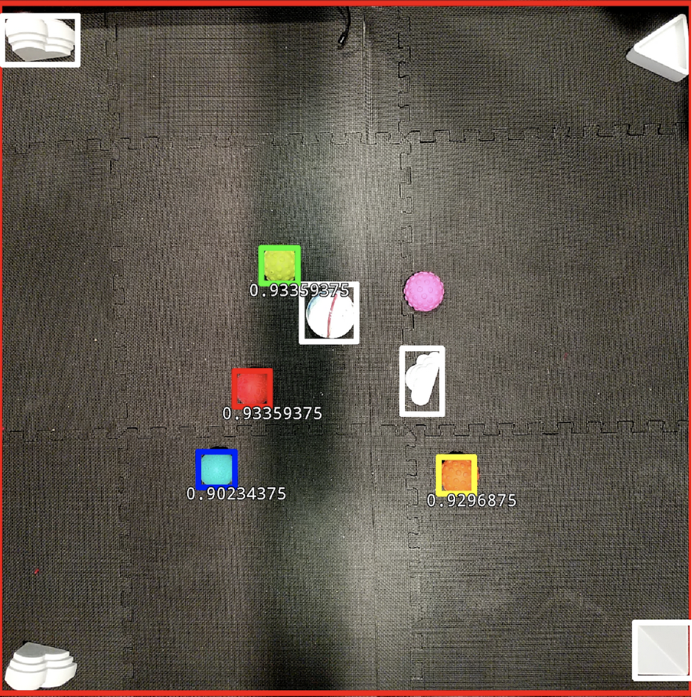
Figure 4 shows a red ball moving during gameplay, with a square bounding box showing where the red ball is in the arena. The red bounding box is slightly off, or behind, the red ball as a result of the slight lag in the object detection process (between 60 and 80 ms). The Commander Model’s direction decision is shown by the red line extending out to the right and slightly upward, telling the robot to change its current heading and go in that direction.
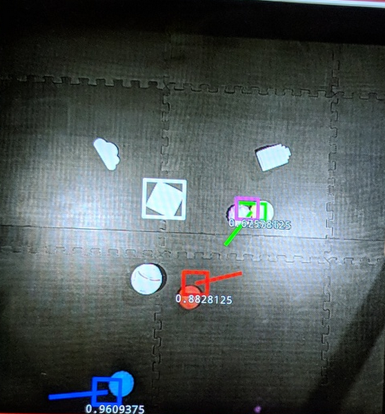

We decided to apply reinforcement learning techniques to train a machine learning model that controls the robot ball’s behaviors. The Sphero API allowed us to specify a heading (in degrees, relative to what the robot considers “forward”) and speed (in percentage). To simplify matters, we had the model control only the heading, and divided 360 degrees into a sequence with 20 degree steps, so our model’s output should be interpreted as 0 degrees, 20 degrees (clockwise), 40 degrees, and so on.
In research literature, many models are built with raw pixels as inputs. Since we already passed the raw images to the Object Detection Model, we decided to use the coordinates (centers of the bounding boxes) as the input of this reinforcement learning model.
Training and evaluation
After preparing data and selecting our initial models, we moved to the actual training and evaluation steps. Based on our Design Goals and Architecture Decisions discussed in our first post, we leveraged the cloud for our training. Google Cloud Machine Learning Engine (CMLE) was used for both Object Detection Model and Commander Model training.
First, we performed a few one-time setup steps locally so that we could train in the cloud.
Second, we generated data and put it into the proper format, as described in the first part in the section above named Gather and Prepare the Data.
Next, we followed the steps outlined in this blog post to train a quantized object detection TensorFlow Lite model.
Once we have our sample app for object detection, we need a custom Object Detection Model trained on our generated data. The blog posts below provide great guides on how to create custom object detection models, and we encourage you to use them as your initial guide:
Dat Tran: How to train your own Object Detector with TensorFlow’s Object Detector API
Training and serving a realtime mobile object detector in 30 minutes with Cloud TPUs
Simulation in the commander model
Early on, we knew it would be very expensive to train this “commander” model with a physical setup, so we planned to use a simulated environment that generates data faster and would not require any manual setup or recharging batteries of the physical robots. To that end we built a custom environment with OpenAI Gym.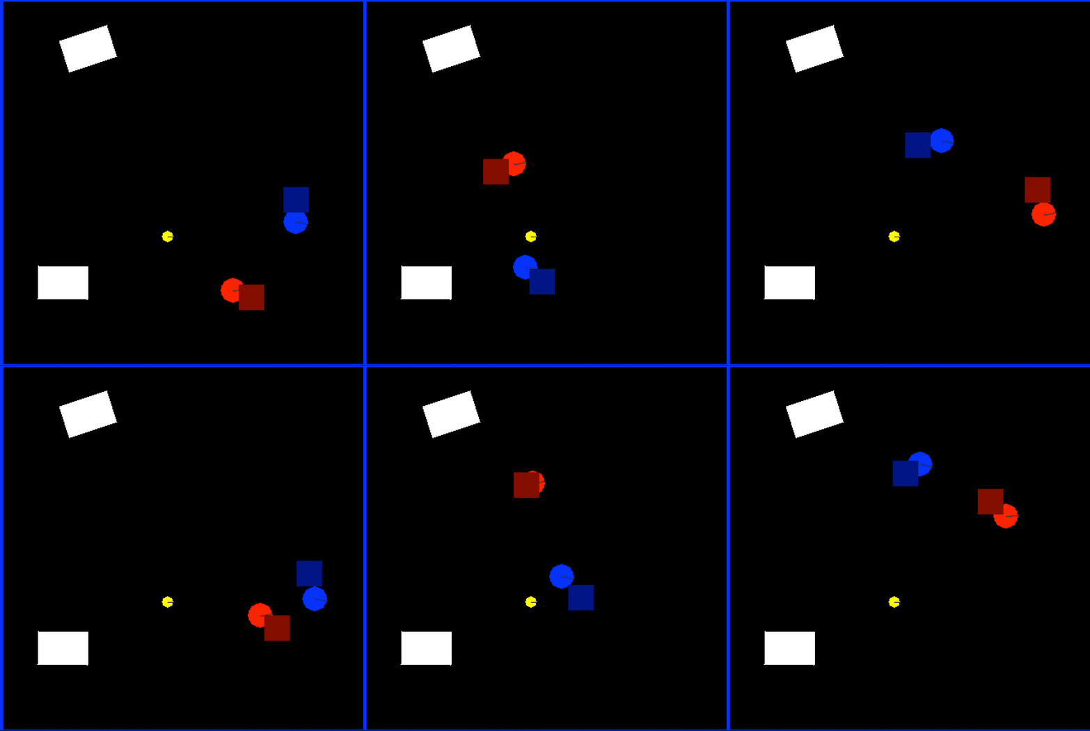

In Figure 6, blue was scripted to always try to go straight at its target, red. Red showed the learned behavior of trying to approach its target (yellow, which does not move) while avoiding blue. The model controlling red was what we use as the Commander Model. The design of the model—having always a target point and a point to avoid—allowed us to use it both as the chaser and the runner in our tag-based games:
When used as a chaser:
Target Point: the nearest legitimate runner
Point to Avoid: the nearest obstacle block
When used as a runner:
Target Point: a home point or a teammate that needs to be unfrozen
Point to Avoid: the chaser
The bounding boxes were always behind the actual positions of the robots due to the Object Detection Model latency, so we forced the Commander Model to make the direction decision based on outdated information: the training data was each robot’s position 5 frames ago (the squares in the Figure 6 video, which have additional noise added to simulate the object detection model’s noisy output), but we configure the model to learn the correct behavior for its current position.
What is this “correct” behavior? In reinforcement learning, the rewards and penalties are often delayed and the attribution of reward/penalty to individual actions is extremely difficult. In our case it seemed reasonable to assign a reward (for red) each time red touched yellow, and a penalty each time red was tagged by blue. All actions taken before either events would be given a discounted reward/penalty based on the eventual outcome. We tried this, and it did not work very well: in some experiments the model was able to learn a good behavior similar to what is shown in the video in Figure 6, but in many other iterations of the same experiment, the model learned to just keep going in the same direction to maximize outcome. We needed a different approach.
We switched to a different approach based on imitation learning, where the model needed to learn by mimicking an expert’s behavior. This did not entirely solve the problem, since we still had to specify the behavior that the model needed to learn, and we really didn’t have time to play the game enough times manually and record the moves as training data.
Eventually, we specified something similar to a potential function on the game field. Imagine the blue robot as the peak of a mountain (which moves!) and yellow as a pit, with gravity naturally ‘pulling’ red towards yellow while rolling away from blue. This approach turned out to be a common technique in robotic path finding.
To make things more realistic, we added an additional “aggressiveness” argument for the Commander Model that controlled the reward function (essentially the balance between how much the model wanted to go towards the pit against how much it wanted to avoid the peak of the mountain. Making changes like these is relatively easy in machine learning compared to, say, modifying the A* path-finding algorithm to incorporate an aggressiveness parameter.
Why did we go through so much trouble to build our model? The chaser’s behavior (“try to tag the nearest runner while avoiding obstacles”) was fairly straightforward to code, and we had a prototype that used the A* path finding algorithm, which worked well. But it was less straightforward to program the runner’s behavior, which involved dynamically deciding a target point for the path finding algorithm based on the chaser’s position. So, we let the machine learning model take care of that dynamic challenge for us.
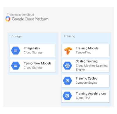

Tools used in training
We wanted to use quantized models to speed up inference, which was very important for the games to proceed in near real-time. But training quantized models could be very slow; some of the training sessions took 7-8 hours to complete with several GPUs. When Cloud TPUs became available, the object detection API research team released training pipelines that utilized TPUs. With a v2-8 TPU pod, we were able to train an object detection model with similar performance in about 3 hours on Cloud Machine Learning Engine.
TPU pods (in beta) became available on Compute Engine when we did our experiments, and with a v2-32 TPU pod, we could finish the same training session in about 1.5 hours. This speedup allowed us much more flexibility when we needed to update the model with different images, and gave us time to work on other parts of the project. This fundamentally changed how we worked, from “start training at the end of day and check results tomorrow” to “start training, go have lunch, and come back to check results.”
We used Cloud Machine Learning Engine (CMLE) to train both our Object Detection Model and Commander Model to take full advantage of the power of the cloud and its many resources. Thus, we could train our models faster using the cloud’s greater quantities of processing power, and also train multiple models at the same time to experiment with different features, all at a very low cost.
The machine learning framework we used to create our models was TensorFlow, and its mobile-focused variant, TensorFlow Lite. We used these because the TensorFlow Research team provided a publicly available model for object detection: MobileNets: Open-Source Models for Efficient On-Device Vision. This meant we only had to supply our training dataset of images and change the config files to use the model, which saved us countless hours in getting a working demo up and running.
Second, TensorFlow let us easily convert our full-size models to TensorFlow Lite, which is optimized for speed, despite the memory and processing constraints of (battery-powered) mobile devices while also maintaining the models’ accuracy. Our quantized Object Detection Model was only 1.6 MB in size. The Commander Model was not quantized, but still only used 2.5 MB of memory. With just a few lines of code in the training loop, we were able to export the commander model in the TensorFlow Lite format without additional conversion.
Next time: On-device prediction
In Part I, we shared the architecture, design principles, and process for the AI in Motion project. In this post, we walked through the key steps of gathering and preparing data, and then selecting and training the models. In our next and final post, we will walk through how we deployed our models on device, and recap how the system works to deliver near real-time predictions and compelling gameplay.
