Going ATOMIC: Clustering and Associating Attacker Activity at Scale
Mandiant
Written by: Matt Berninger
At FireEye, we work hard to detect, track, and stop attackers. As part of this work, we learn a great deal of information about how various attackers operate, including details about commonly used malware, infrastructure, delivery mechanisms, and other tools and techniques. This knowledge is built up over hundreds of investigations and thousands of hours of analysis each year. At the time of publication, we have 50 APT or FIN groups, each of which have distinct characteristics. We have also collected thousands of uncharacterized 'clusters' of related activity about which we have not yet made any formal attribution claims. While unattributed, these clusters are still useful in the sense that they allow us to group and track associated activity over time.
However, as the information we collect grows larger and larger, we realized we needed an algorithmic method to assist in analyzing this information at scale, to discover new potential overlaps and attributions. This blog post will outline the data we used to build the model, the algorithm we developed, and some of the challenges we hope to tackle in the future.
The Data
As we detect and uncover malicious activity, we group forensically-related artifacts into 'clusters'. These clusters indicate actions, infrastructure, and malware that are all part of an intrusion, campaign, or series of activities which have direct links. These are what we call our "UNC" or "uncategorized" groups. Over time, these clusters can grow, merge with other clusters, and potentially 'graduate' into named groups, such as APT33 or FIN7. This graduation occurs only when we understand enough about their operations in each phase of the attack lifecycle and have associated the activity with a state-aligned program or criminal operation.
For every group, we can generate a summary document that contains information broken out into sections such as infrastructure, malware files, communication methods, and other aspects. Figure 1 shows a fabricated example with the various 'topics' broken out. Within each 'topic' – such as 'Malware' – we have various 'terms', which have associated counts. These numbers indicate how often we have recorded a group using that 'term'.
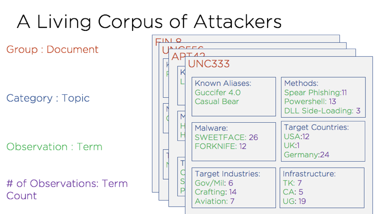

Figure 1: Example group 'documents' demonstrating how data about groups is recorded
The Problem
Our end goal is always to merge a new group either into an existing group once the link can be proven, or to graduate it to its own group if we are confident it represents a new and distinct actor set. These clustering and attribution decisions have thus far been performed manually and require rigorous analysis and justification. However, as we collect increasingly more data about attacker activities, this manual analysis becomes a bottleneck. Clusters risk going unanalyzed, and potential associations and attributions could slip through the cracks. Thus, we now incorporate a machine learning-based model into our intelligence analysis to assist with discovery, analysis, and justification for these claims.
The model we developed began with the following goals:
- Create a single, interpretable similarity metric between groups
- Evaluate past analytical decisions
- Discover new potential matches
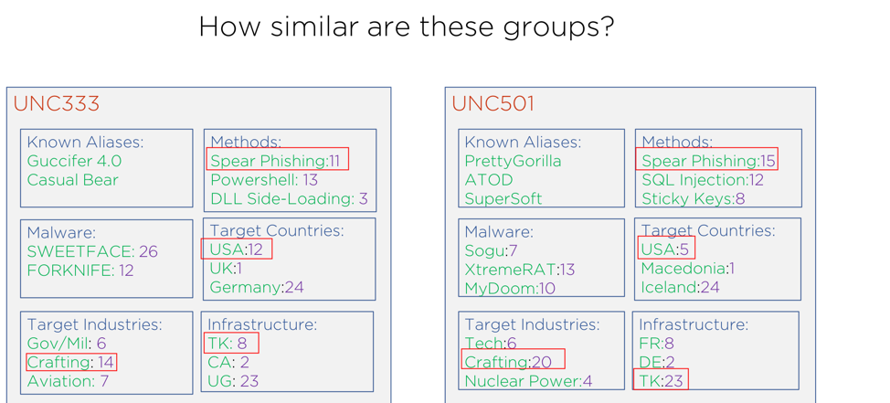

Figure 2: Example documents highlighting observed term overlaps between two groups
The Model
This model uses a document clustering approach, familiar in the data science realm and often explained in the context of grouping books or movies. Applying the approach to our structured documents about each group, we can evaluate similarities between groups at scale.
First, we decided to model each topic individually. This decision means that each topic will result in its own measure of similarity between groups, which will ultimately be aggregated to produce a holistic similarity measure.
Here is how we apply this to our documents.
Within each topic, every distinct term is transformed into a value using a method called term frequency -inverse document frequency, or TF-IDF. This transformation is applied to every unique term for every document + topic, and the basic intuition behind it is to:
- Increase importance of the term if it occurs often with the document.
- Decrease the importance of the term if it appears commonly across all documents.
This approach rewards distinctive terms such as custom malware families – which may appear for only a handful of groups – and down-weights common things such as 'spear-phishing', which appear for the vast majority of groups.
Figure 3 shows an example of TF-IDF being applied to a fictional "UNC599" for two terms: mal.sogu and mal.threebyte. These terms indicate the usages of SOGU and THREEBYTE within the 'malware' topic and thus we calculate their value within that topic using TF-IDF. The first (TF) value is how often those terms appeared as a fraction of all malware terms for the group. The second value (IDF) is the inverse of how frequently those terms appear across all groups. Additionally, we take the natural log of the IDF value, to smooth the effects of highly common terms – as you can see in the graph, when the value is close to 1 (very common terms), the log evaluates to near-zero, thus down-weighting the final TF x IDF value. Unique values have a much higher IDF, and thus result in higher values.
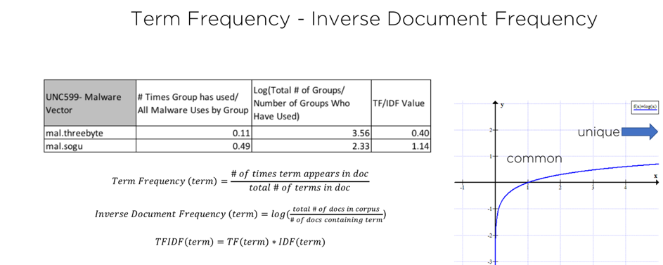

Figure 3: Breakdown of TF-IDF metric when evaluated for a single group in regard to malware
Once each term has been given a score, each group is now reflected as a collection of distinct topics, and each topic is a vector of scores for the terms it contains. Each vector can be conceived as an arrow, detailing the 'direction' that group is 'pointing'within that topic.
Within each topic space, we can then evaluate the similarity of various groups using another method – Cosine Similarity. If, like me, you did not love trigonometry – fear not! The intuition is simple. In essence, this is a measure of how parallel two vectors are. As seen in Figure 4, to evaluate two groups' usage of malware, we plot their malware vectors and see if they are pointing in the same direction. More parallel means they are more similar.
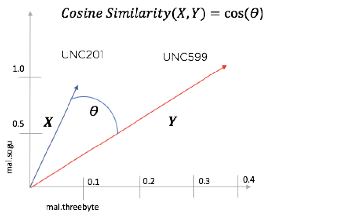

Figure 4: Simplified breakdown of Cosine Similarity metric when applied to two groups in the malware 'space'
One of the nice things about this approach is that large and small vectors are treated the same – thus, a new, relatively small UNC cluster pointing in the same direction as a well-documented APT group will still reflect a high level of similarity. This is one of the primary use cases we have, discovering new clusters of activity with high similarity to already established groups.
Using TF-IDF and Cosine Similarity, we can now calculate the topic-specific similarities for every group in our corpus of documents. The final step is to combine these topic similarities into a single, aggregate metric (Figure 5). This single metric allows us to quickly query our data for 'groups similar to X' or 'similarity between X and Y'. The question then becomes: What is the best way to build this final similarity?
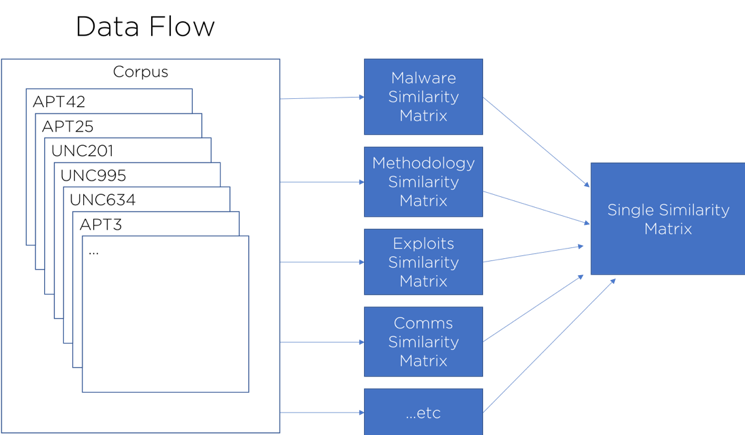

Figure 5: Overall model flow diagram showing individual topic similarities and aggregation in to final similarity matrix
The simplest approach is to take an average, and at first that’s exactly what we did. However, as analysts, this approach did not sync well with analyst intuition. As analysts, we feel that some topics matter more than others. Malware and methodologies should be more important than say, server locations or target industries...right? However, when challenged to provide custom weightings for each topic, it was impossible to find an objective weighting system, free from analyst bias. Finally, we thought: "What if we used existing, known data to tell us what the right weights are?" In order to do that, we needed a lot of known – or "labeled" – examples of both similar and dissimilar groups.
Building a Labeled Dataset
At first our concept seemed straightforward: We would find a large dataset of labeled pairs, and then fit a regression model to accurately classify them. If successful, this model should give us the weights we wanted to discover.
Figure 6 shows some graphical intuition behind this approach. First, using a set of ‘labeled’ pairs, we fit a function which best predicts the data points.
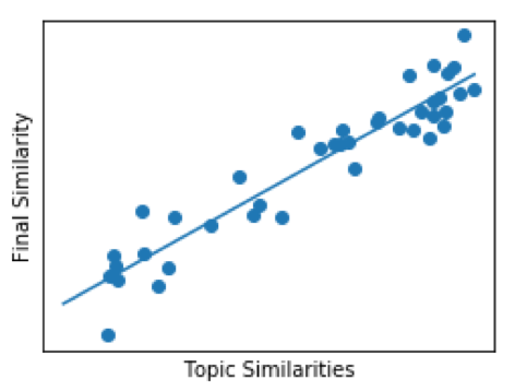

Figure 6: Example Linear regression plot—in reality we used a Logistic Regression, but showing a linear model to demonstrate the intuition
Then, we use that same function to predict the aggregate similarity of un-labeled pairs (Figure 7).
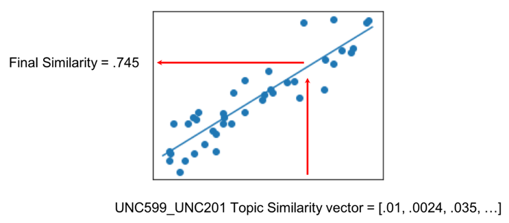

Figure 7: Example of how we used the trained model to predict final similarity from individual topic similarities.
However, our data posed a unique problem in the sense that only a tiny fraction of all potential pairings had ever been analyzed. These analyses happened manually and sporadically, often the result of sudden new information from an investigation finally linking two groups together. As a labeled dataset, these pairs were woefully insufficient for any rigorous evaluation of the approach. We needed more labeled data.
Two of our data scientists suggested a clever approach: What if we created thousands of 'fake' clusters by randomly sampling from well-established APT groups? We could therefore label any two samples that came from the same group as definitely similar, and any two from separate groups as not similar (Figure 8). This gave us the ability to synthetically generate the labeled dataset we desperately needed. Then, using a linear regression model, we were able to elegantly solve this 'weighted average' problem rather than depend on subjective guesses.


Figure 8: Example similarity testing with 'fake' clusters derived from known APT groups
Additionally, these synthetically created clusters gave us a dataset upon which to test various iterations of the model. What if we remove a topic? What if we change the way we capture terms? Using a large labeled dataset, we can now benchmark and evaluate performance as we update and improve the model.
To evaluate the model, we observe several metrics:
- Recall for synthetic clusters we know come from the same original group – how many do we get right/wrong? This evaluates the accuracy of a given approach.
- For individual topics, the 'spread' between the calculated similarity of related and unrelated clusters. This helps us identify which topics help separate the classes best.
- The accuracy of a trained regression model, as a proxy for the 'signal' between similar and dissimilar clusters, as represented by the topics. This can help us identify overfitting issues as well.
Operational Use
In our daily operations, this model serves to augment and assist our intelligence experts. Presenting objective similarities, it can challenge biases and introduce new lines of investigation not previously considered. When dealing with thousands of clusters and new ones added every day from analysts around the globe, even the most seasoned and aware intel analyst could be excused for missing a potential lead. However, our model is able to present probable merges and similarities to analysts on demand, and thus can assist them in discovery.
Upon deploying this to our systems in December 2018, we immediately found benefits. One example is outlined in this blog post about potentially destructive attacks. Since then we have been able to inform, discover, or justify dozens of other merges.
Future Work
Like all models, this one has its weaknesses and we are already working on improvements. There is label noise in the way we manually enter information from investigations. There is sometimes 'extraneous' data about attackers that is not (yet) represented in our documents. Most of all, we have not yet fully incorporated the 'time of activity' and instead rely on 'time of recording'. This introduces a lag in our representation, which makes time-based analysis difficult. What an attacker has done lately should likely mean more than what they did five years ago.
Taking this objective approach and building the model has not only improved our intel operations, but also highlighted data requirements for future modeling efforts. As we have seen in other domains, building a machine learning model on top of forensic data can quickly highlight potential improvements to data modeling, storage, and access. Further information on this model can also be viewed in this video, from a presentation at the 2018 CAMLIS conference.
We have thus far enjoyed taking this approach to augmenting our intelligence model and are excited about the potential paths forward. Most of all, we look forward to the modeling efforts that help us profile, attribute, and stop attackers.
