Reverse Engineering the Analyst: Building Machine Learning Models for the SOC
Mandiant
Written by: Matt Berninger, Awalin Sopan
Many cyber incidents can be traced back to an original alert that was either missed or ignored by the Security Operations Center (SOC) or Incident Response (IR) team. While most analysts and SOCs are vigilant and responsive, the fact is they are often overwhelmed with alerts. If a SOC is unable to review all the alerts it generates, then sooner or later, something important will slip through the cracks.
The core issue here is scalability. It is far easier to create more alerts than to create more analysts, and the cyber security industry is far better at alert generation than resolution. More intel feeds, more tools, and more visibility all add to the flood of alerts. There are things that SOCs can and should do to manage this flood, such as increasing automation of forensic tasks (pulling PCAP and acquiring files, for example) and using aggregation filters to group alerts into similar batches. These are effective strategies and will help reduce the number of required actions a SOC analyst must take. However, the decisions the SOC makes still form a critical bottleneck. This is the “Analyze/ Decide” block in Figure 1.


Figure 1: Basic SOC triage stages
In this blog post, we propose machine learning based strategies to help mitigate this bottleneck and take back control of the SOC. We have implemented these strategies in our FireEye Managed Defense SOC, and our analysts are taking advantage of this approach within their alert triaging workflow. In the following sections, we will describe our process to collect data, capture alert analysis, create a model, and build an efficacy workflow – all with the ultimate goal of automating alert triage and freeing up analyst time.
Reverse Engineering the Analyst
Every alert that comes into a SOC environment contains certain bits of information that an analyst uses to determine if the alert represents malicious activity. Often, there are well-paved analytical processes and pathways used when evaluating these forensic artifacts over time. We wanted to explore if, in an effort to truly scale our SOC operations, we could extract these analytical pathways, train a machine to traverse them, and potentially discover new ones.
Think of a SOC as a self-contained machine that inputs unlabeled alerts and outputs the alerts labeled as “malicious” or “benign”. How can we capture the analysis and determine that something is indeed malicious, and then recreate that analysis at scale? In other words, what if we could train a machine to make the same analytical decisions as an analyst, within an acceptable level of confidence?
Basic Supervised Model Process
The data science term for this is a “Supervised Classification Model”. It is “supervised” in the sense that it learns by being shown data already labeled as benign or malicious, and it is a “classification model” in the sense that once it has been trained, we want it to look at a new piece of data and make a decision between one of several discrete outcomes. In our case, we only want it to decide between two “classes” of alerts: malicious and benign.
In order to begin creating such a model, a dataset must be collected. This dataset forms the “experience” of the model, and is the information we will use to “train” the model to make decisions. In order to supervise the model, each unit of data must be labeled as either malicious or benign, so that the model can evaluate each observation and begin to figure out what makes something malicious versus what makes it benign. Typically, collecting a clean, labeled dataset is one of the hardest parts of the supervised model pipeline; however, in the case of our SOC, our analysts are constantly triaging (or “labeling”) thousands of alerts every week, and so we were lucky to have an abundance of clean, standardized, labeled alerts.
Once a labeled dataset has been defined, the next step is to define “features” that can be used to portray the information resident in each alert. A “feature” can be thought of as an aspect of a bit of information. For example, if the information is represented as a string, a natural “feature” could be the length of the string. The central idea behind building features for our alert classification model was to find a way to represent and record all the aspects that an analyst might consider when making a decision.
Building the model then requires choosing a model structure to use, and training the model on a subset of the total data available. The larger and more diverse the training data set, generally the better the model will perform. The remaining data is used as a “test set” to see if the trained model is indeed effective. Holding out this test set ensures the model is evaluated on samples it has never seen before, but for which the true labels are known.
Finally, it is critical to ensure there is a way to evaluate the efficacy of the model over time, as well as to investigate mistakes so that appropriate adjustments can be made. Without a plan and a pipeline to evaluate and retrain, the model will almost certainly decay in performance.
Feature Engineering
Before creating any of our own models, we interviewed experienced analysts and documented the information they typically evaluate before making a decision on an alert. Those interviews formed the basis of our feature extraction. For example, when an analyst says that reviewing an alert is “easy”, we ask: “Why? And what helps you make that decision?” It is this reverse engineering of sorts that gives insight into features and models we can use to capture analysis.
For example, consider a process execution event. An alert on a potentially malicious process execution may contain the following fields:
- Process Path
- Process MD5
- Parent Process
- Process Command Arguments
While this may initially seem like a limited feature space, there is a lot of useful information that one can extract from these fields.
Beginning with the process path of, say, “C:\windows\temp\m.exe”, an analyst can immediately see some features:
- The process resides in a temporary folder: C:\windows\temp\
- The process is two directories deep in the file system
- The process executable name is one character long
- The process has an .exe extension
- The process is not a “common” process name
While these may seem simple, over a vast amount of data and examples, extracting these bits of information will help the model to differentiate between events. Even the most basic aspects of an artifact must be captured in order to “teach” the model to view processes the way an analyst does.
The features are then encoded into a more discrete representation, similar to this:
Another important feature to consider about a process execution event is the combination of parent process and child process. Deviation from expected “lineage” can be a strong indicator of malicious activity.
Say the parent process of the aforementioned example was ‘powershell.exe’. Potential new features could then be derived from the concatenation of the parent process and the process itself: ‘powershell.exe_m.exe’. This functionally serves as an identity for the parent-child relation and captures another key analysis artifact.
The richest field, however, is probably the process arguments. Process arguments are their own sort of language, and language analysis is a well-tread space in predictive analytics.
We can look for things including, but not limited to:
- Network connection strings (such as ‘http://’, ‘https://’, ‘ftp://’).
- Base64 encoded commands
- Reference to Registry Keys (‘HKLM’, ‘HKCU’)
- Evidence of obfuscation (ticks, $, semicolons) (read Daniel Bohannon’s work for more)
The way these features and their values appear in a training dataset will define the way the model learns. Based on the distribution of features across thousands of alerts, relationships will start to emerge between features and labels. These relationships will then be recorded in our model, and ultimately used to influence the predictions for new alerts. Looking at distributions of features in the training set can give insight into some of these potential relationships.
For example, Figure 2 shows how the distribution of Process Command Length may appear when grouping by malicious (red) and benign (blue).
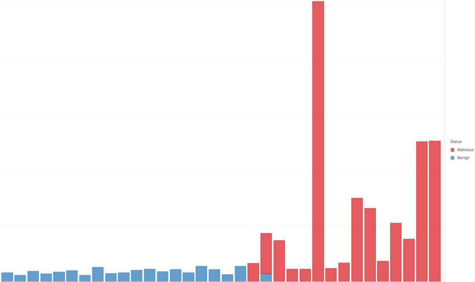

Figure 2: Distribution of Process Event alerts grouped by Process Command Length
This graph shows that over a subset of samples, the longer the command length, the more likely it is to be malicious. This manifests as red on the right and blue on the left. However, process length is not the only factor.
As part of our feature set, we also thought it would be useful to approximate the “complexity” of each command. For this, we used “Shannon entropy”, a commonly used metric that measures the degree of randomness present in a string of characters.
Figure 3 shows a distribution of command entropy, broken out into malicious and benign. While the classes do not separate entirely, we can see that for this sample of data, samples with higher entropy generally have a higher chance of being malicious.
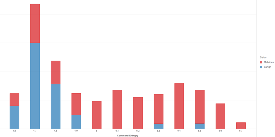

Figure 3: Distribution of Process Event alerts grouped by entropy
Model Selection and Generalization
Once features have been generated for the whole dataset, it is time to use them to train a model. There is no perfect procedure for picking the best model, but looking at the type of features in our data can help narrow it down. In the case of a process event, we have a combination of features represented as strings and numbers. When an analyst evaluates each artifact, they ask questions about each of these features, and combine the answers to estimate the probability that the process is malicious.
For our use case, it also made sense to prioritize an ‘interpretable’ model – that is, one that can more easily expose why it made a certain decision about an artifact. This way analysts can build confidence in the model, as well as detect and fix analytical mistakes that the model is making. Given the nature of the data, the decisions analysts make, and the desire for interpretability, we felt that a decision tree-based model would be well-suited for alert classification.
There are many publicly available resources to learn about decision trees, but the basic intuition behind a decision tree is that it is an iterative process, asking a series of questions to try to arrive at a highly confident answer. Anyone who has played the game “Twenty Questions” is familiar with this concept. Initially, general questions are asked to help eliminate possibilities, and then more specific questions are asked to narrow down the possibilities. After enough questions are asked and answered, the ‘questioner’ feels they have a high probability of guessing the right answer.
Figure 4 shows an example of a decision tree that one might use to evaluate process executions.
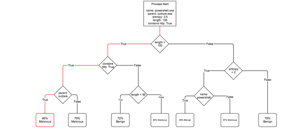

Figure 4: Decision tree for deciding whether an alert is benign or malicious
For the example alert in the diagram, the “decision path” is marked in red. This is how this decision tree model makes a prediction. It first asks: “Is the length greater than 100 characters?” If so, it moves to the next question “Does it contain the string ‘http’?” and so on until it feels confident in making an educated guess. In the example in Figure 4, given that 95 percent of all the training alerts traveling this decision path were malicious, the model predicts a 95 percent chance that this alert will also be malicious.
Because they can ask such detailed combinations of questions, it is possible that decision trees can “overfit”, or learn rules that are too closely tied to the training set. This reduces the model’s ability to “generalize” to new data. One way to mitigate this effect is to use many slightly different decision trees and have them each “vote” on the outcome. This “ensemble” of decision trees is called a Random Forest, and it can improve performance for the model when deployed in the wild. This is the algorithm we ultimately chose for our model.
How the SOC Alert Model Works
When a new alert appears, the data in the artifact is transformed into a vector of the encoded features, with the same structure as the feature representations used to train the model. The model then evaluates this “feature vector” and applies a confidence level for the predicted label. Based on thresholds we set, we can then classify the alert as malicious or benign.


Figure 5: An alert presented to the analyst with its raw values captured
As an example, the event shown in Figure 5 might create the following feature values:
- Parent Process: ‘wscript’
- Command Entropy: 5.08
- Command Length =103
Based on how they were trained, the trees in the model each ask a series of questions of the new feature vector. As the feature vector traverses each tree, it eventually converges on a terminal “leaf” classifying it as either benign or malicious. We can then evaluate the aggregated decisions made by each tree to estimate which features in the vector played the largest role in the ultimate classification.
For the analysts in the SOC, we then present the features extracted from the model, showing the distribution of those features over the entire dataset. This gives the analysts insight into “why” the model thought what it thought, and how those features are represented across all alerts we have seen. For example, the “explanation” for this alert might look like:
- Command Entropy = 5.08 > 4.60: 51.73% Threat
- occuranceOfChar “\”= 9.00 > 4.50: 64.09% Threat
- occuranceOfChar:“)” (=0.00) <= 0.50: 78.69% Threat
- NOT processTree=”cmd.exe_to_cscript.exe”: 99.6% Threat
Thus, at the time of analysis, the analysts can see the raw data of the event, the prediction from the model, an approximation of the decision path, and a simplified, interpretable view of the overall feature importance.
How the SOC Uses the Model
Showing the features the model used to reach the conclusion allows experienced analysts to compare their approach with the model, and give feedback if the model is doing something wrong. Conversely, a new analyst may learn to look at features they may have otherwise missed: the parent-child relationship, signs of obfuscation, or network connection strings in the arguments. After all, the model has learned on the collective experience of every analyst over thousands of alerts. Therefore, the model provides an actionable reflection of the aggregate analyst experience back to the SOC, so that each analyst can transitively learn from their colleagues.
Additionally, it is possible to write rules using the output of the model as a parameter. If the model is particularly confident on a subset of alerts, and the SOC feels comfortable automatically classifying that family of threats, it is possible to simply write a rule to say: “If the alert is of this type, AND for this malware family, AND the model confidence is above 99, automatically call this alert bad and generate a report.” Or, if there is a storm of probable false positives, one could write a rule to cull the herd of false positives using a model score below 10.
How the Model Stays Effective
The day the model is trained, it stops learning. However, threats – and therefore alerts – are constantly evolving. Thus, it is imperative to continually retrain the model with new alert data to ensure it continues to learn from changes in the environment.
Additionally, it is critical to monitor the overall efficacy of the model over time. Building an efficacy analysis pipeline to compare model results against analyst feedback will help identify if the model is beginning to drift or develop structural biases. Evaluating and incorporating analyst feedback is also critical to identify and address specific misclassifications, and discover potential new features that may be necessary.
To accomplish these goals, we run a background job that updates our training database with newly labeled events. As we get more and more alerts, we periodically retrain our model with the new observations. If we encounter issues with accuracy, we diagnose and work to address them. Once we are satisfied with the overall accuracy score of our retrained model, we store the model object and begin using that model version.
We also provide a feedback mechanism for analysts to record when the model is wrong. An analyst can look at the label provided by the model and the explanation, but can also make their own decision. Whether they agree with the model or not, they can input their own label through the interface. We store this label provided by the analyst along with any optional explanation given by them regarding the explanation.
Finally, it should be noted that these manual labels may require further evaluation. As an example, consider a commodity malware alert, in which network command and control communications were sinkholed. An analyst may evaluate the alert, pull back triage details, including PCAP samples, and see that while the malware executed, the true threat to the environment was mitigated. Since it does not represent an exigent threat, the analyst may mark this alert as ‘benign’. However, the fact that it was sinkholed does not change that the artifacts of execution still represent malicious activity. Under different circumstances, this infection could have had a negative impact on the organization. However, if the benign label is used when retraining the model, that will teach the model that something inherently malicious is in fact benign, and potentially lead to false negatives in the future.
Monitoring efficacy over time, updating and retraining the model with new alerts, and evaluating manual analyst feedback gives us visibility into how the model is performing and learning over time. Ultimately this helps to build confidence in the model, so we can automate more tasks and free up analyst time to perform tasks such as hunting and investigation.
Conclusion
A supervised learning model is not a replacement for an experienced analyst. However, incorporating predictive analytics and machine learning into the SOC workflow can help augment the productivity of analysts, free up time, and ensure they utilize investigative skills and creativity on the threats that truly require expertise.
This blog post outlines the major components and considerations of building an alert classification model for the SOC. Data collection, labeling, feature generation, model training, and efficacy analysis must all be carefully considered when building such a model. FireEye continues to iterate on this research to improve our detection and response capabilities, continually improve the detection efficacy of our products, and ultimately protect our clients.
The process and examples shown discussed in this post are not mere research. Within our FireEye Managed Defense SOC, we use alert classification models built using the aforementioned processes to increase our efficiency and ensure we apply our analysts’ expertise where it is needed most. In a world of ever increasing threats and alerts, increasing SOC efficiency may mean the difference between missing and catching a critical intrusion.
Acknowledgements
A big thank you to Seth Summersett and Clara Brooks.
***
The FireEye ICE Data Science Team is a small, highly trained team of data scientists and engineers, focused on delivering impactful capabilities to our analysts, products, and customers. ICE-DS is always looking for exceptional candidates interested in researching and solving difficult problems in cybersecurity. If you’re interested, check out Mandiant careers.
