PyTorch/XLA: Performance debugging on Cloud TPU VM: Part III
Vaibhav Singh
Group Product Manager
This article is the final in the three part series to explore the performance debugging ecosystem of PyTorch/XLA on Google Cloud TPU VM. In the first part, we introduced the key concept to reason about the training performance using PyTorch/XLA profiler and ended with an interesting performance bottleneck we encountered in the Multi-Head-Attention (MHA) implementation in PyTorch 1.8. In the second part, we began with another implementation of MHA introduced in PyTorch 1.9 which solved the performance bottleneck and identified an example of Dynamic Graph during evaluation using the profiler and studied a possible trade-off between CompileTime penalty with ‘device-to-host’ transfers.
In this part, we shift gears to server-side profiling. Recall from client and server terminology introduced in the first part, the server side functionality refers to all the computations that happen at TPU Runtime (aka XRT server) and beyond (on TPU device). Often, the objective of such an analysis is to peek into performance of a certain op, or a certain section of your model on TPUs. PyTorch/XLA facilitates this with user annotations which can be inserted in the source code and can be visualized as a trace using Tensorboard.
Environment setup
We continue to use the mmf (multimodal framework) example used in the first two parts. If you are starting with this part, please refer to the Environment Setup section of part-1 to create a TPU VM and continue from the TensorBoard Setup described in this post. We recap the commands here for easy access
Creation of TPU VM instance (if not already created):
Here is the command to SSH into the instance once the instance is created.
TensorBoard setup
Notice the ssh flag argument for ssh tunneled port forwarding. This allows you to connect to the application server listening to port 9009 via localhost:9009 on your own browser. To setup TensorBoard version correctly and avoid conflict with other local version, please uninstall the existing TensorBoard version first:
In the current context the application server is the TensorBoard instance listening to port 9009:
This will start the TensorBoard server accessible via localhost:9009 on your browser. Notice that no profiling data is collected yet. Follow the instructions from the user guide to open the PROFILE view localhost:9009.
Training setup
We anchor to the PyTorch / XLA 1.9 environment for this case study.
Update alternative (make python3 default):
Configure environment variables:
MMF training environment
The MMF (Multimodal Training Framework) library developed by Meta Research is built to help researchers easily experiment with the models for multi-modal (text/image/audio) learning problems. As described in the roadmap we will use the UniTransformer model for this case study. We will begin by cloning and installing the mmf library (specific hash chosen for reproducibility purposes).
Before we install the mmf library in developer mode, please make the following modifications in the requirement.txt (such that the existing PyTorch environment is not overridden when mmf is installed):
Apply the following patch for validate_batch_sizes method (Specific to the commit selected for this article):
Install the mmf library in developer mode:
Trace API
The PyTorch/XLA profiler provides two primary APIs (StepTrace, Trace) to help you analyze the different segments of your code through annotations which can later be visualized using TensorBoard. To use StepTrace or Trace, first a profiler server needs to be started.
Starting profiler server
In the following code snippet, we modified the main method (mmf_cli/run.py) to introduce the start_server (<port_number>) call. Notice that the server object returned by this method will only persist if captured in a variable. Therefore server = xp.start_server(3294) will start a profiler server that persists throughout the training. However if we only called start server xp.start_server(3294) without any assignment, the server object does not persist and you will not be able to interact with the server (later on we will request the server via TensorBoard to capture the profile for a given period of time.)
Make a note of the port number used as the argument to start_server call (in this case 3294). We will use this when communicating with the profiler server in the later sections.
Insert traces annotations
Once the mmf library is installed in the developer mode, we can make changes to the source code as shown below to follow this case study.
In the following code snippet we illustrate StepTrace and Trace annotations. The former introduces a named context (called Training_Step) within which we introduce a few more nested named contexts to capture forward, backward and update times through the latter annotations.
Note that xp refers to import torch_xla.debug.profiler as xp as illustrated in earlier code snippet.
Once the training starts we can capture these annotations onto the trace by either the xp.trace method or TensorBoard Profiler’s Capture Profile feature. In this case study we will use the TensorBoard feature for interactive and iterative profile capture. In development test settings xp.trace can be used to capture the profile data into a TensorBoard logdir, however be cautioned that trace data can quickly grow and therefore trace call should only be active for a reasonable time period.
Start TensorBoard
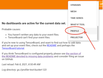
Recall the TensorBoard setup instructions shared in the earlier section (TensorBoard Setup). You started the TensorBoard server at port 9009. And when you ssh into the TPU VM instance we forwarded port 9009 of our localhost to 9009 of the TPU VM. Once you open localhost:9009 in your browser, you will see the following UI:
Note: If you do not see Profile options in the drop-down menu, please check the TensorBoard version and ensure that the profiler plugin was installed as instructed in the setup section.
Start training
Start the training using the same script that you used earlier with one modification. We change the distributed world size to 8 (for all-reduce visualization in the trace).
Once the training is underway you should begin to see the following log snippet:
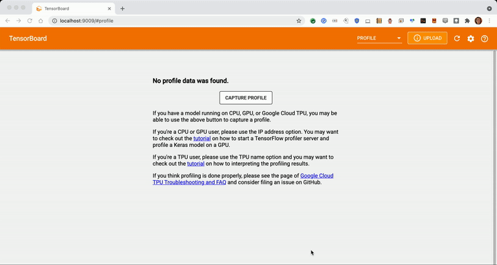
Capture profile
Form TensorBoard UI which you started earlier, Click ‘Capture Profile’ and specify the localhost:3294 (the same port number you specified in the start_server call):
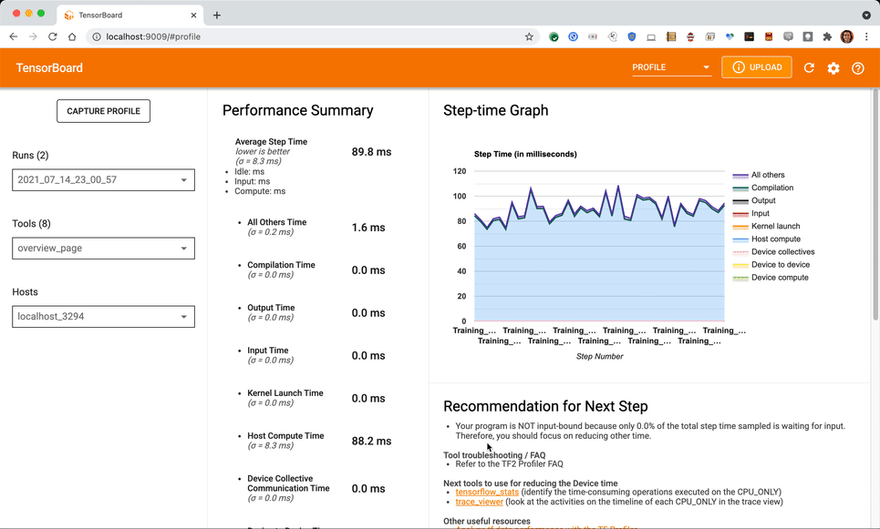
Once the capture is complete you should see an overview page similar to the following (if more than one training step is captured in the trace, else the overview page may be blank, since it requires at least one training step completed to provide any input pipeline recommendations.
In this case-study, we will focus on the trace view for details about other views. (For memory profiler, pod viewer, etc. please refer to the TensorBoard profiler documentation.) Some of these functionalities are not fully supported by TPU VM at the time of writing this article.
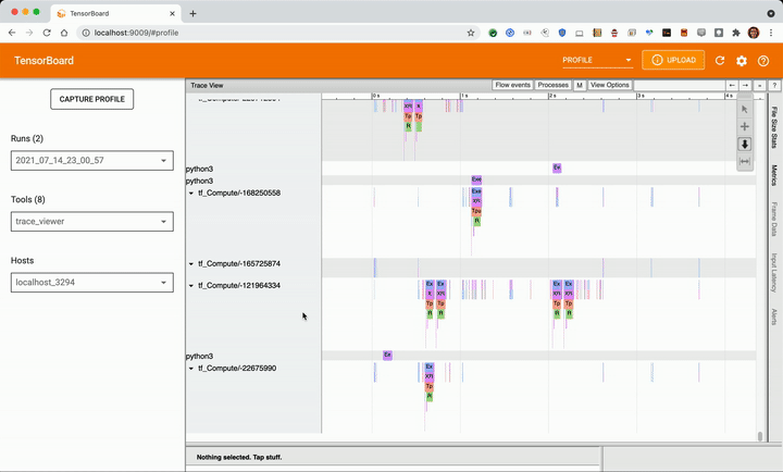
Navigate to the annotations in the Trace Viewer
In the Trace Viewer, Traces collected from all the device i.e. TPU processes and all the host i.e. CPU processes are displayed. You can use the search bar and scroll down to find the annotations you have introduced in the source code:
Understanding Trace
The following picture shows the annotations that we created in the code snippet example:
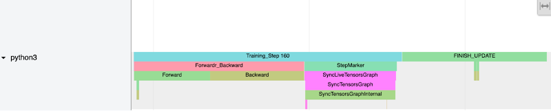
Notice the Training Step trace and sub-traces forward and backward pass. These annotations on the CPU process trace Indicate the time spent in the forward backward pass (IR graph) traversal. In case forward or backward passes force early execution (unlowered op or value fetch) you will notice forward or backward traces broken and interspersed multiple times with StepMarker. StepMarker is an in-built annotation which corresponds to implicit or explicit mark_step() call.
Notice also the FINISH_UPDATE trace. In the mmf code, this corresponds to reduce gradients and update operations. We notice another host process which which is starting TPUExecute function call:
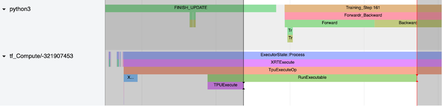
If we create a window from the TPUExecute to the end of the RunExecutable trace we expect to see graph execution and all-reduce traces on the device (scroll back up to the top).
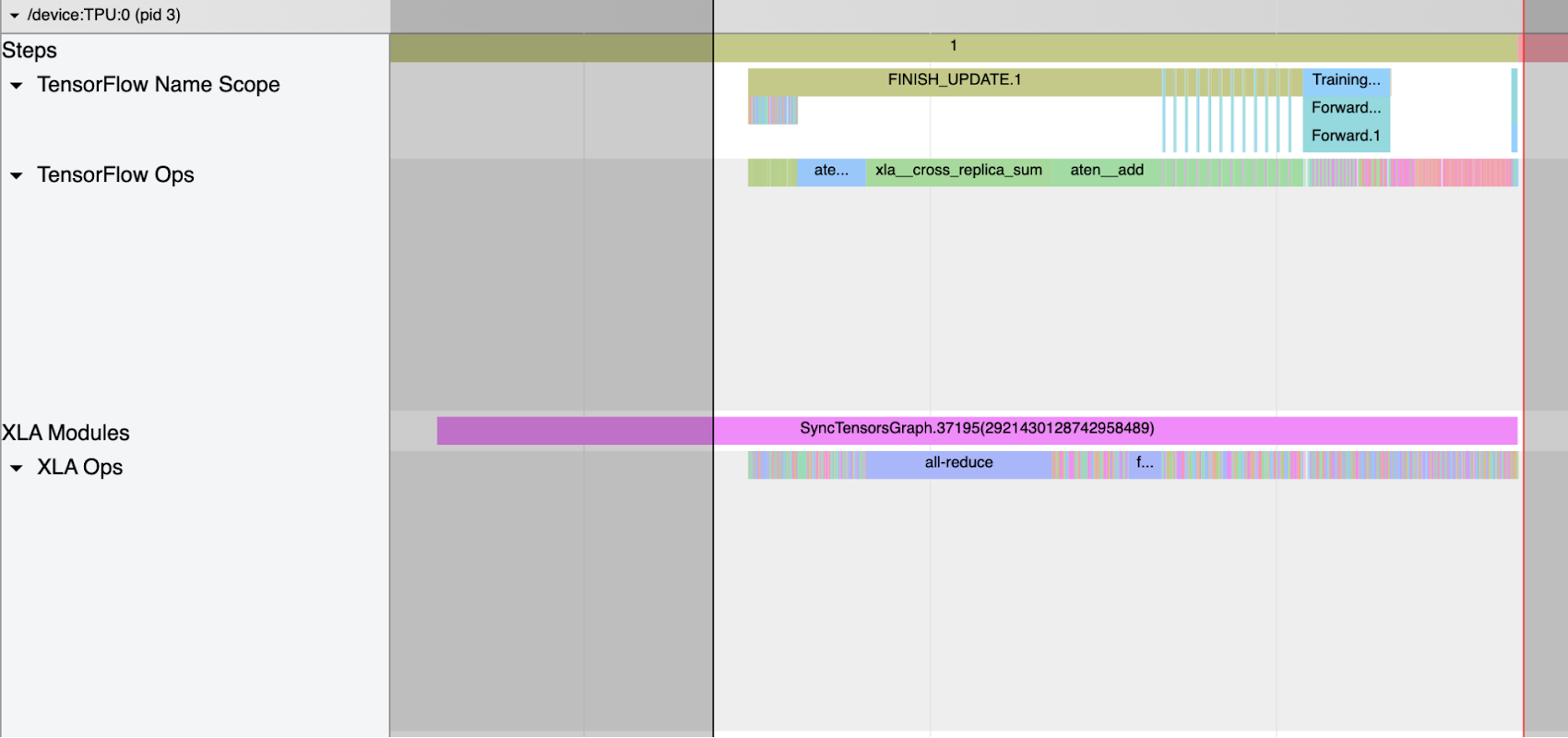
Notice the all_reduce xla_op and corresponding all reduce cross replica sum appearing in tensorflow op. Tensorflow Name Scope and Tensorflow Ops show up in the trace when XLA_HLO_DEBUG is enabled (ref code snippet in Start Training section). It shows the annotation propagated to the HLO (High Level Operations) graph.
Notice also the gaps on the device trace. The duty cycle (i.e. the fraction of annotated trace per cycle) is the fraction of time spent on graph execution on the device. To investigate the gaps it’s often a good practice to select the gap duration using the trace viewer window tool and then examine the CPU traces to understand what other operations are being executed in that period. For example, in the following trace we select the 72.143ms period where no device trace is observed:
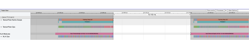
Examining the same period across cpu traces (zoomed in view), we notice three main time chunks:
1. Overlapping with the IR generation (backward pass) of the next step, followed by StepMarker (mark_step()) call. MarkStep signals to PyTorch/XLA that the IR graph traversed thus far is to be executed now. If it’s a new graph, it will be compiled and optimized first (you will notice longer StepMarker trace and also separate process traces annotated “xxyy” ):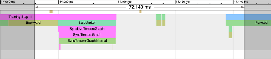
2. Graph/Data is Transferred to the Server (i.e transfer from host to TPU device):
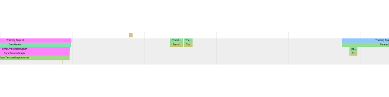
In the case of TPU VM transfer-to-server is expected to be an inexpensive operation.
3. XRTExecute is initiated which loads the program (graph) from cache if found or loads the input graph and eventually triggers TPU execution. (Details of XRTExecute, allocation, load program, signature etc is outside the scope of this case-study).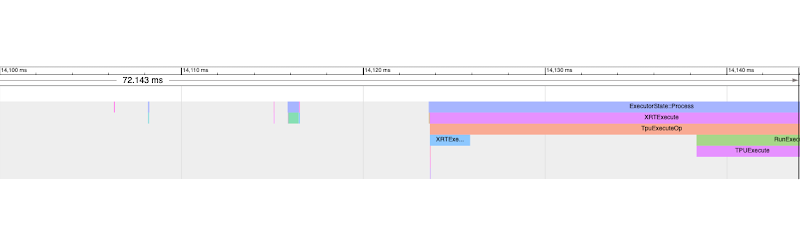
Notice also that the IR generation for the following step has already begun while the current step is executed on TPU.
In summary, the gaps in device trace are good regions to investigate. Apart from the three chunks or scenarios above, it can also be due to in-efficient data pipeline. In order to investigate you can also add annotations to data-loading parts of the code and then inspect it in the trace wrt to device execution. For a good pipeline data loading and transfer-to-server should overlap with device execution. If this is not the case, the device will be idle for some time waiting for data and this would be input pipeline bottleneck.
Annotation propagation
Since PyTorch/XLA training involves IR graph translated into HLO graph which is then compiled and optimized further by the runtime and those optimization do not preserve the initial graph structure, these annotations when propagated to HLO graphs and beyond (enabled by XLA_HLO_DEBUG=1) do not appear in the same order. For example consider the following trace (zooming into the trace shown above):

This window does not correspond to multiple forward and backward traces in the host process (you notice gaps in the trace when neither forward or train step tags appear), still we notice Training_Step, Forward and FINISH_UPDATE traces are interspersed here. And this is because the graph to which initial annotation is propagated has undergone multiple optimization passes.
Conclusion
Annotation propagation into the host and device traces using the profiler API provides a powerful mechanism to analyze the performance of your training. In this case study we did not deduce any optimizations to reduce training time from this analysis but only introduced it for educational purposes. These optimizations can improve efficiency, TPU utilization, duty cycle, training ingestion throughput and such.
Next steps
As an exercise, we recommend the readers to repeat the analysis performed in this study with log_interval set to 1. This exercise will accentuate device-to-host transfer costs and the effects of some of the changes discussed to optimize the training performance.
This concludes the part-3 of our three part series on performance debugging. We reviewed the basic performance concepts and command line debug in part-1. In Part-1 we investigated a transformer based model training which was slow due to too frequent device to host transfers. Part-1 ended with an exercise for the reader(s) to improve the training performance. In Part-2 we started with the solution of the part-1 exercise and examined another common pattern of performance degradation, the dynamic graph. And finally, in this post we took a deeper dive into performance analysis using annotations and tensorboard trace viewer. We hope that the concepts presented in this series would be helpful for the readers to debug their training runs effectively using PyTorch/XLA profiler and derive actionable insights to improve the training performance. The reader is encouraged to experiment with their own models and apply and learn the concepts presented here.
Acknowledgements
The author would like to thank Jordan Totten, Rajesh Thallam, Karl Weinmeister and Jack Cao (Google) for your patience and generosity. Each one of you provided numerous feedback without which this post would be riddled with annoying errors. Special thanks to Jordan for patiently testing the case studies presented in this series, for finding many bugs, and providing valuable suggestions. Thanks to Joe Spisak, Geeta Chauhan (Meta) and Shauheen Zahirazami and Zak Stone (Google) for your encouragement, especially for the feedback to split what would have been too long a post for anyone to read. Thanks to Ronghong Hu (Meta AI) for the feedback and questions on the early revisions which made, especially, the trace discussion much more accessible and helpful. And finally to Amanpreet Singh (Meta AI), the author of MMF framework, for your inputs in various debugging discussions, case study selection and for your inputs in building the TPU support in MMF, without your help this series would not be possible.


