A deep dive into Spanner’s query optimizer

Spanner is a fully managed, distributed relational database that provides unlimited scale, global consistency, and up to five 9s availability. It was originally built to address Google’s needs to scale out Online Transaction Processing (OLTP) workloads without losing the benefits of strong consistency and familiar SQL that developers rely on. Today, Cloud Spanner is used in financial services, gaming, retail, health care, and other industries to power mission-critical workloads that need to scale without downtime. 

Like most modern relational databases, Spanner uses a query optimizer to find efficient execution plans for SQL queries. When a developer or a DBA writes a query in SQL, they describe the results they want to see, rather than how to access or update the data. This declarative approach allows the database to select different query plans depending on a wide variety of signals, such as the size and shape of the data and available indexes. Using these inputs, the query optimizer finds an execution plan for each query.

You can see a graphical view of a plan from the Cloud Console. It shows the intermediate steps that Spanner uses to process the query. For each step, it details where time and resources are spent and how many rows each operation produces. This information is useful for identifying bottlenecks and to test changes to queries, indexes, or the query optimizer itself.

How does the Spanner query optimizer work?

Let’s start with the following example schema and query, using Spanner’s Google Standard SQL dialect. 

Schema:

Query:

When Spanner receives a SQL query, it is parsed into an internal representation known as relational algebra. This is essentially a tree structure in which each node represents some operation of the original SQL. For example, every table access will appear as a leaf node in the tree and every join will be a binary node with its two inputs being the relations that it joins. The relational algebra for our example query looks like this:

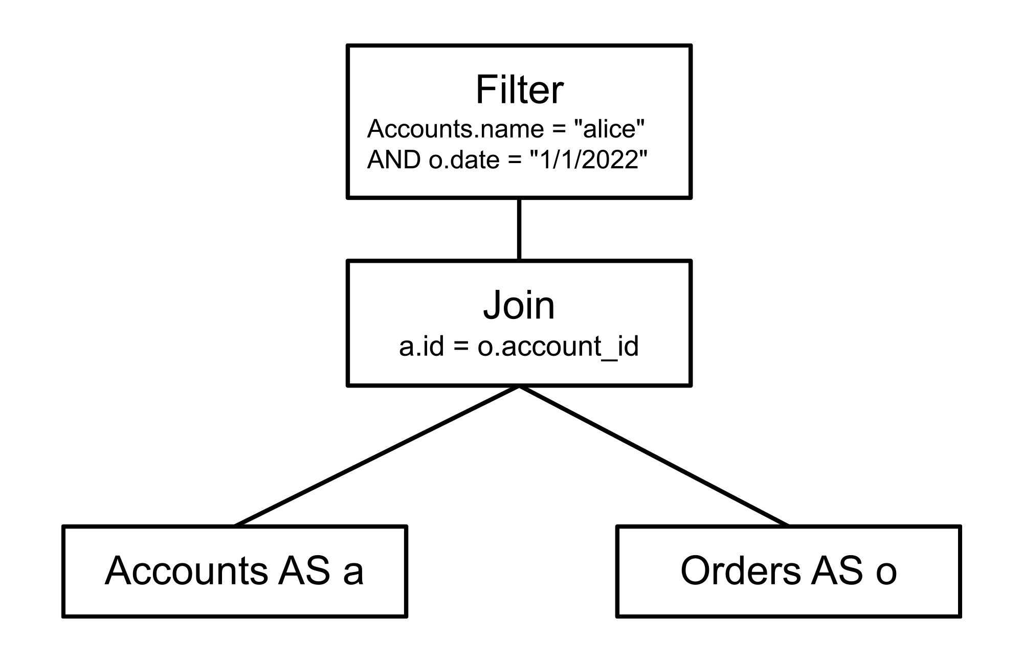
The query optimizer has two major stages that it uses to generate an efficient execution plan based on this relational algebra: heuristic optimization and cost-based optimization. Heuristic optimization, as the name indicates, applies heuristics, or pre-defined rules, to improve the plan. Those heuristics are manifested in several dozen replacement rules which are a subclass of algebraic transformation rule. Heuristic optimization improves the logical structure of the query in ways that are essentially guaranteed to make the query faster, such as moving filter operations closer to the data they filter, converting outer joins to inner joins where possible, and removing any redundancy in the query. However, many important decisions about an execution plan cannot be made heuristically, so they are made in the second stage, cost-based optimization, in which the query planner uses estimates of latency to choose between available alternatives. Let’s first look at how replacement rules work in heuristic optimization as a prelude to cost-based optimization.

A replacement rule has two steps: a pattern matching step and an application step. In the pattern matching step, the rule attempts to match a fragment of the tree with some predefined pattern. When it finds a match, the second step is to replace the matched fragment of the tree with some other predefined fragment of tree. The next section provides a straightforward example of a replacement rule in which a filter operation is moved, or pushed, beneath a join.

Example of a replacement rule

This rule pushes a filter operation closer to the data that it is filtering. The rationale for doing this is two-fold: 

• Pushing filters closer to the relevant data reduces the volume of data to be processed later in the pipeline
• Placing a filter closer to the table creates an opportunity to use an index on the filtered column(s) to scan only the rows that qualify the filter.

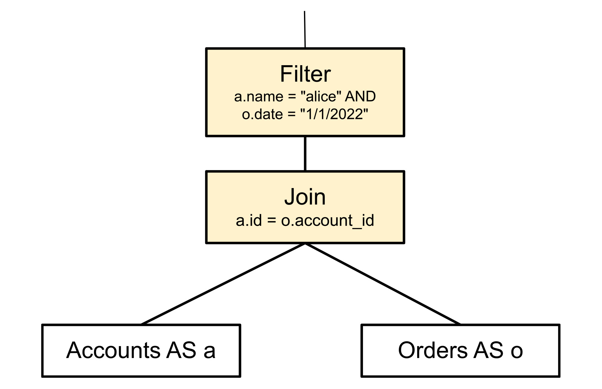
The rule matches the pattern of a filter node with a join node as its child. Details such as table names and the specifics of the filter condition are not part of the pattern matching. The essential elements of the pattern are just the filter with the join beneath it, the two shaded nodes in the tree illustrated below. The two leaf nodes in the picture need not actually be leaf nodes in the real tree, they themselves could be joins or other operations. They are included in the illustration simply to show context.

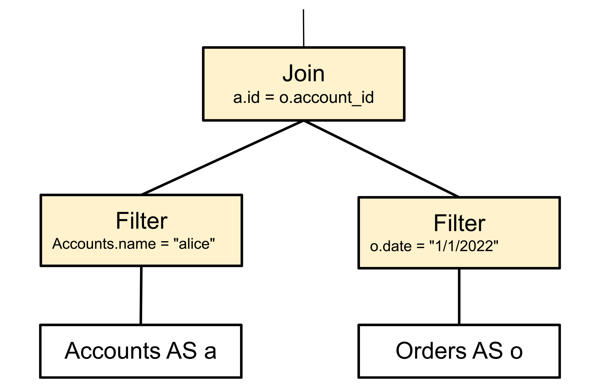
The replacement rule rearranges the tree, as shown below, replacing the filter and join nodes. This changes how the query is executed, but does not change the results. The original filter node is split in two, with each predicate pushed to the relevant sides of the join from which the referenced columns are produced. This tells the query execution to filter the rows before they’re joined, so the join doesn’t have to handle rows that would later be rejected.

Cost-based optimization

There are big decisions about an execution plan for which no effective heuristics exist. These decisions must be made with an understanding of how different alternatives will perform. Hence the second stage of the query optimizer is the cost-based optimizer. In this stage, the optimizer makes decisions based on estimates of the latencies, or the costs, of different alternatives. Cost-based optimization provides a more dynamic approach than heuristics alone. It uses the size and shape of the data to calculate multiple execution plans. To developers, this means more efficient plans out-of-the-box and less hand tuning. 

The architectural backbone of this stage is the extensible optimizer generator framework known as Cascades. Cascades is the foundation of multiple industry and open-source query optimizers. This optimization stage is where the more impactful decisions are made, such as which indexes to use, what join order to use, and what join algorithms to use. Cost-based optimization in Spanner uses several dozen algebraic transformation rules. However, rather than being replacement rules, they are exploration and implementation rules. These classes of rules have two steps. As for replacement rules, the first step is a pattern matching step. However, rather than replacing the original matched fragment with some fixed alternative fragment, in general they provide multiple alternatives to the original fragment. 

Example of an exploration rule

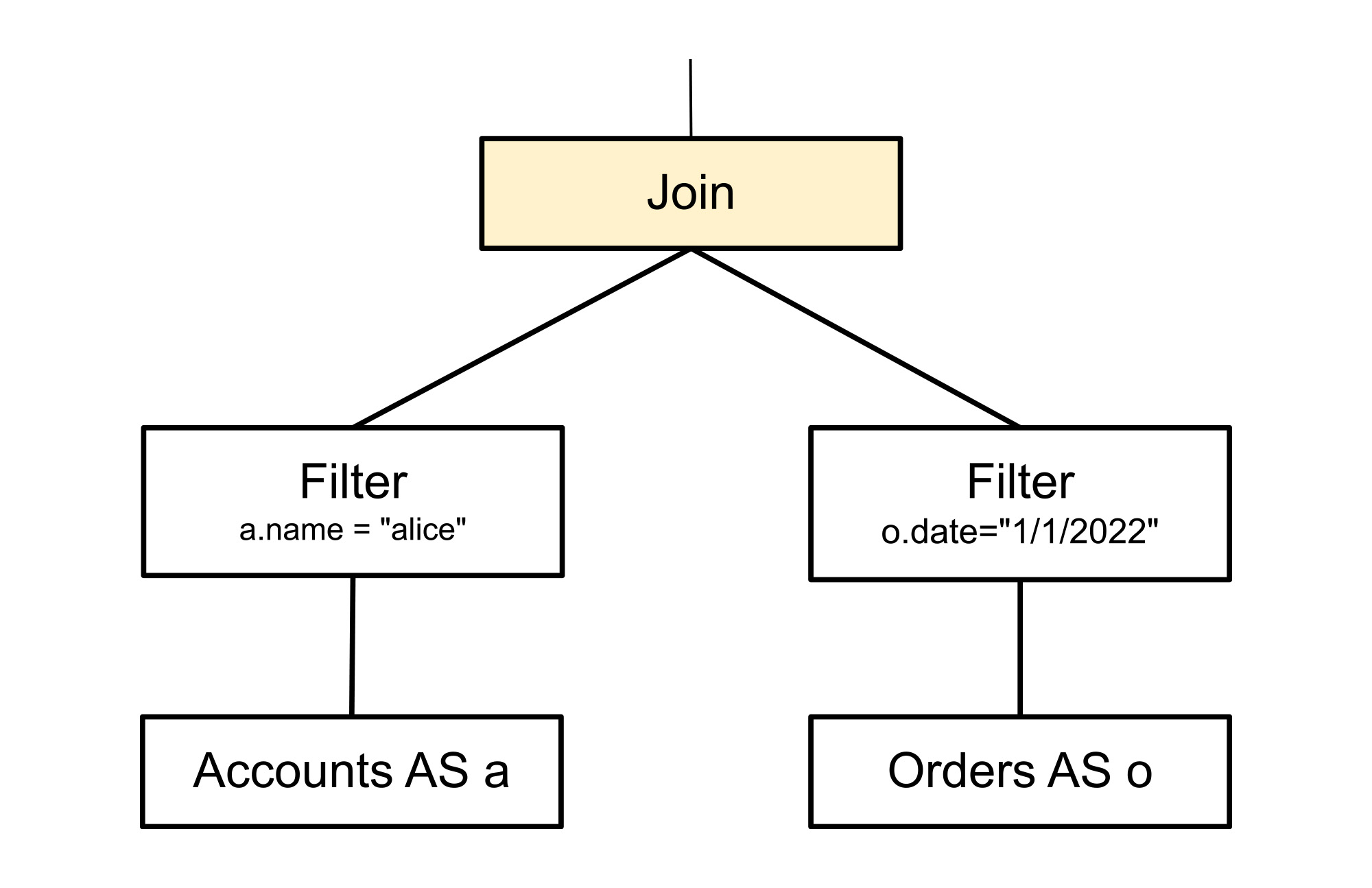
The following exploration rule matches a very simple pattern, a join. It generates one additional alternative in which the inputs to the join have been swapped. Such a transformation doesn’t change the meaning of the query because relational joins are commutative, in much the same way that arithmetic addition is commutative. The content of unshaded nodes in the following illustration do not matter to the rule and they are shown only to provide context.

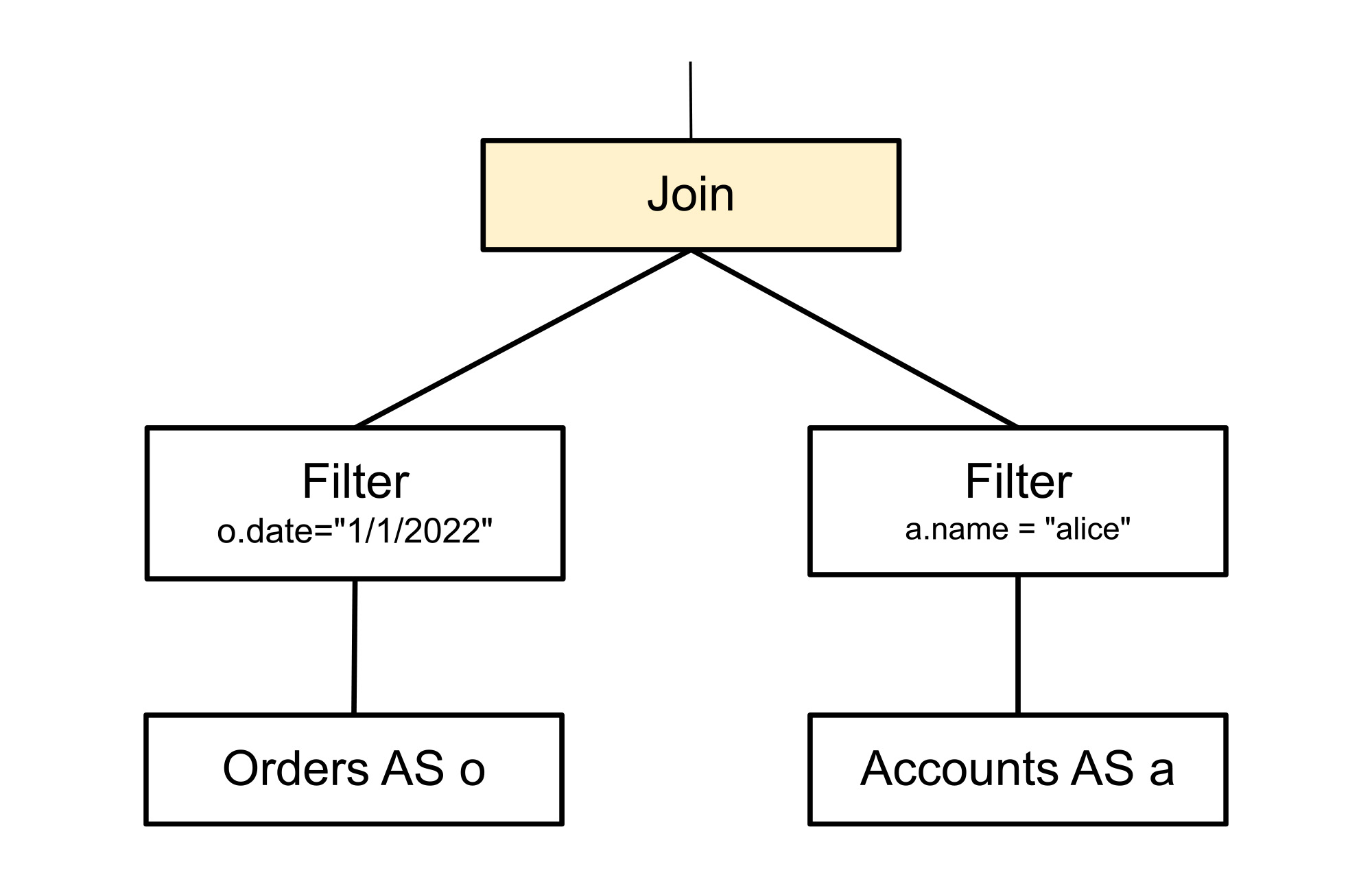
The following tree shows the new fragment that is generated. Specifically, the shaded node below is created as an available alternative to the original shaded node. It does not replace the original node. The unshaded nodes have swapped positions in the new alternative but are not modified in any way. They now have two parents instead of one. At this point, the query is no longer represented as a simple tree but as a directed acyclic graph (DAG). The rationale for this transformation is that the ordering of the inputs to a join can profoundly impact its performance. Typically, a join will perform faster if the first input that it accesses, which for Spanner means left side, is the smaller one. However, the optimal choice will also depend on many other factors, including the available indexes and the ordering requirements of the query.

Example of an implementation rule

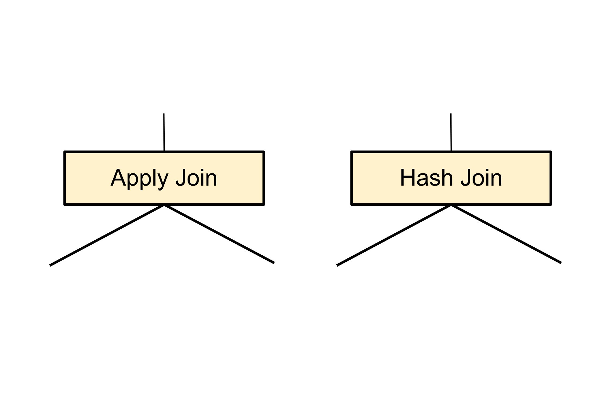
Once again the following implementation rule pattern matches a join but this time it generates two alternatives: apply join and hash join. These two alternatives replace the original logical join operation.

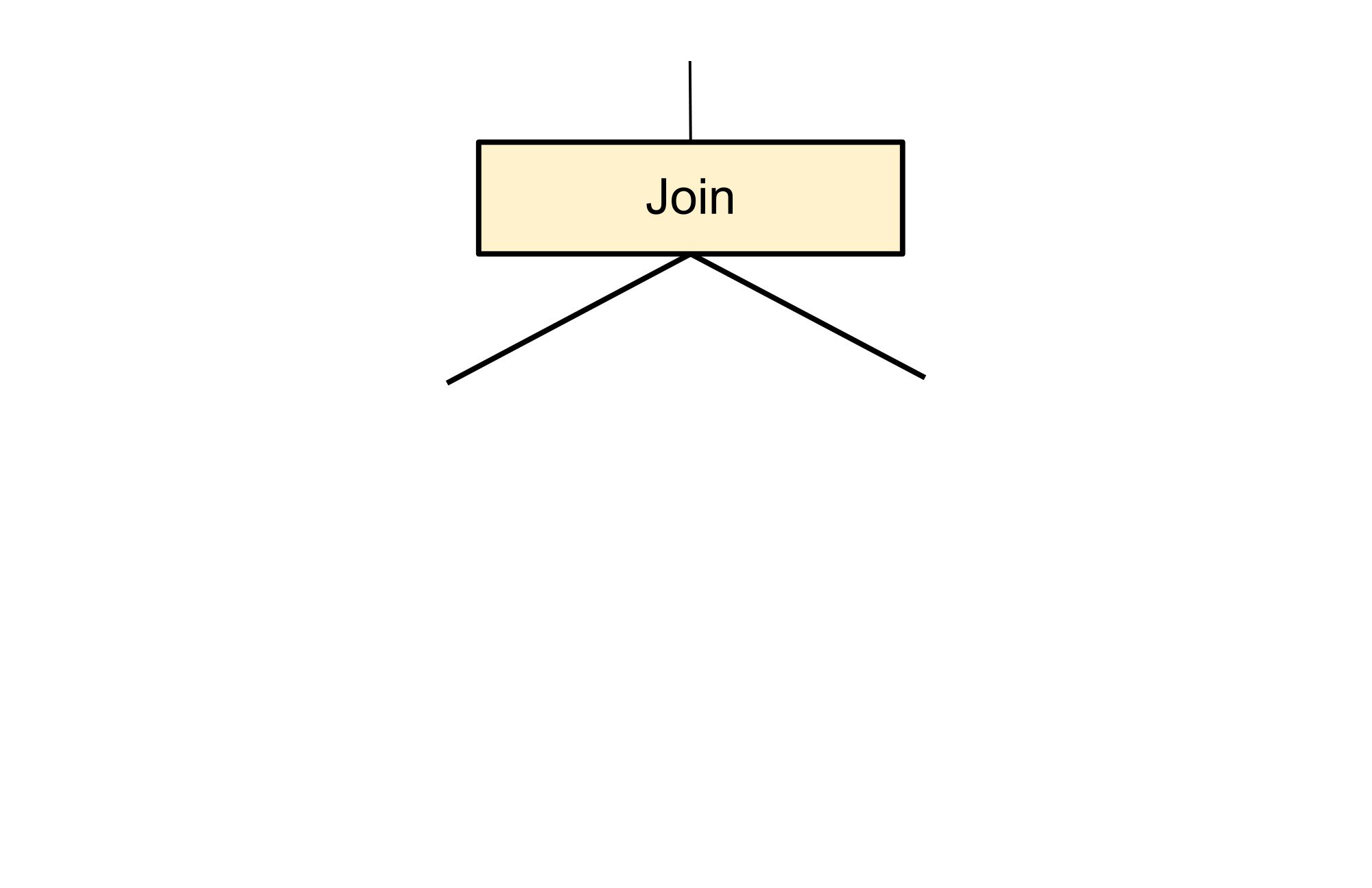
The above fragment will be replaced by the following two alternatives which are two possible ways of executing a join.

Cascades and the evaluation engine

The Cascades engine manages the application of the exploration and implementation rules and all the alternatives they generate. It calls an evaluation engine to estimate the latency of fragments of execution plans and, ultimately, complete execution plans. The final plan that it selects is the plan with the lowest total estimated latency according to the evaluation engine. 

The optimizer considers many factors when estimating the latency of a node in an execution plan. These include exactly what operation the node performs (e.g. hash join, sort etc.), the storage medium when accessing data, and how the data is partitioned. But chief among those factors is an estimate of how many rows will enter the node and how many rows will exit the node. To estimate those row counts Spanner uses built-in statistics that characterize the actual data.

Why does the query optimizer need statistics?

How does the query optimizer select which strategies to use in assembling the plan? One important signal is descriptive statistics about the size, shape, and cardinality of the data. As part of regular operation, Spanner periodically samples each database to estimate metrics like distinct values, distributions of values, number of NULLs, data size for each column, and some combination of columns. These metrics are called optimizer statistics.

To demonstrate how statistics help the optimizer pick a query plan, let’s consider a simple example using the previously described schema. 

Let’s look at the optimal plan for this query:

There are two possible execution strategies that the query optimizer will consider:

1. Base table plan: read all rows from Accounts and filter out those whose name is different from the value of parameter, @p.

2. Index plan: Read the rows of accounts where name is equal to @p from the AccountsByName index. Then join the set with the Accounts table to fetch the age column.

Let’s compare these visually in the plan viewer:

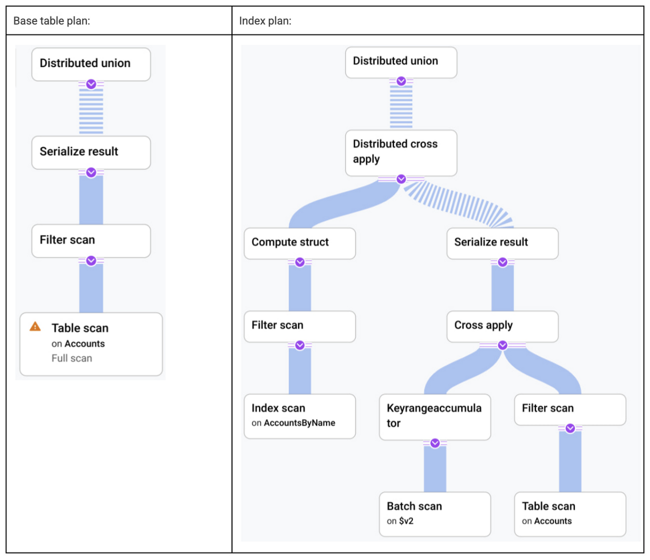
Interestingly, even for this simple example there is no query plan that is obviously best. The optimal query plan depends on filter selectivity, or how many rows in Accounts match the condition. For the sake of simplicity let’s suppose that 10 rows in Accounts have name = "alice", while the remaining 45,000 rows have name = "bob". The latency of the query with each plan might look something like, using the fastest index plan for alice as our baseline:

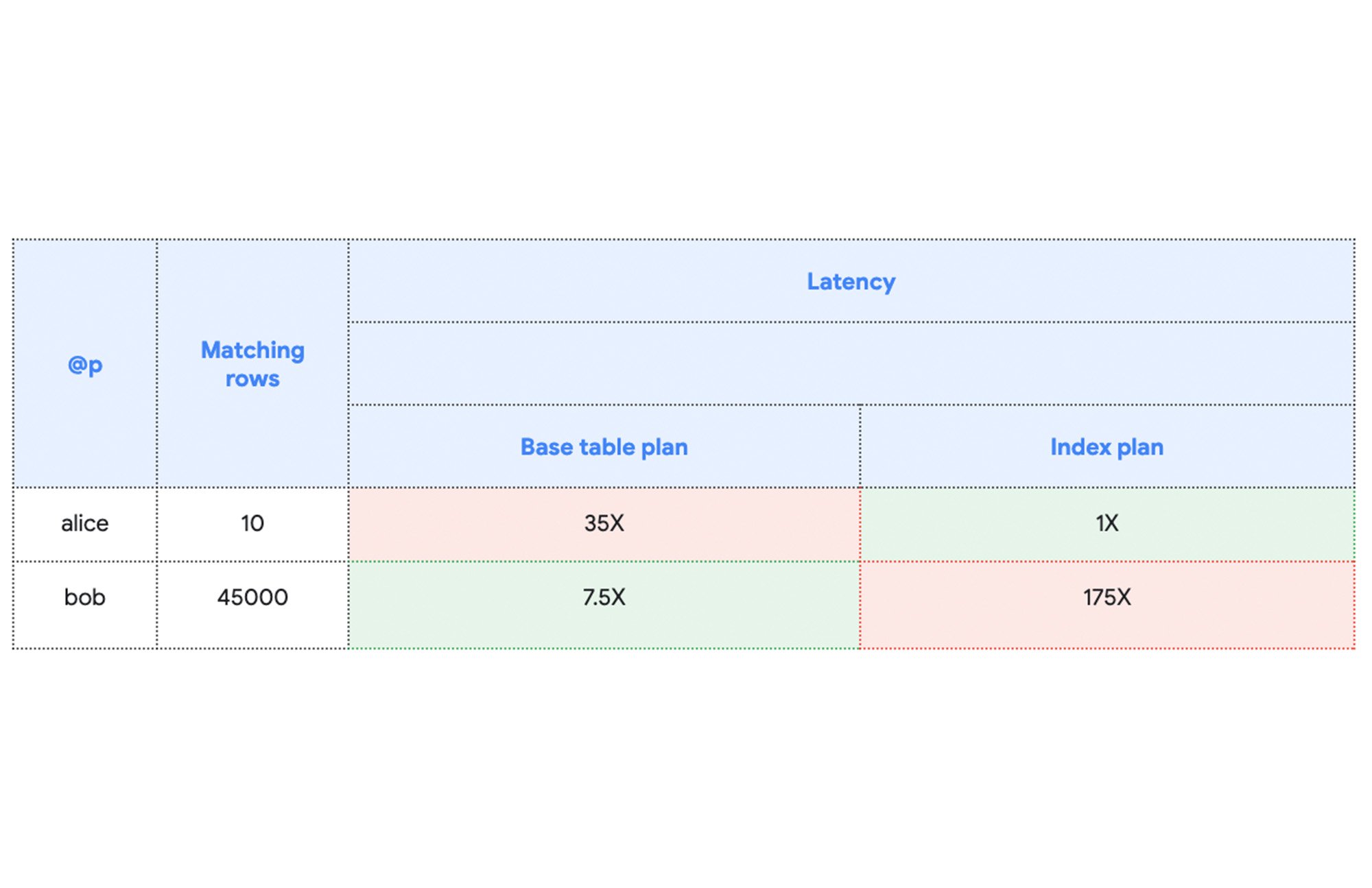
We can see in this simple example that the optimal query plan choice depends on the actual data stored in the database and the specific conditions in the query, in this example, up to 175 times faster. The statistics describe the shape of data in the database and help Spanner estimate which plan would be preferable for the query.

Optimizer statistics collection

Spanner automatically updates the optimizer statistics to reflect the changes to the database schema and data. A background process recalculates them roughly every three days. The query optimizer will automatically use the latest version as input to query planning.

In addition to automatic collection, you can also manually refresh the optimizer statistics using the ANALYZE DDL statement. This is particularly useful when a database’s schema or data are changing frequently, such as in a development environment, where you’re changing tables or indexes, or in production when large amounts of data are changing, such as in a new product launch or a large data clean-up. 

The optimizer statistics include:

• Approximate number of rows in each table.
• Approximate number of distinct values of each column and each composite key prefix (including index keys). For example if we have table T with key {a, b, c}, Spanner will store the number of distinct values for {a}, {a, b} and {a, b, c}.
• Approximate number of NULL, empty and NaN values in each column.
• Approximate minimum, maximum and average value byte size for each column.
• Histogram describing data distribution in each column. The histogram captures both ranges of values and frequent values.

For example the Accounts table in the previous example has 45,010 total rows. The id column has 45,010 distinct values (since it is a key) and the name column has 2 distinct values (“alice” and “bob”).

Histograms store a small sample of the column data to denote the boundaries of histogram bins. Disabling garbage collection for a statistics package will delay wipeout of this data. 

Query optimizer versioning

The Spanner development team is continuously improving the query optimizer. Each update broadens the class of queries where the optimizer picks the more efficient execution plan. The log of optimizer updates is available in the public documentation.

We are doing extensive testing to ensure that new query optimizer versions select better query plans than before. Because of this, most workloads should not have to worry about query optimizer rollouts. By staying current they automatically inherit improvements as we enable them.

There is a small chance, however, that an optimizer update will flip a query plan to a less performant one. If this happens, it will show up as a latency increase for the workload. 

Cloud Spanner provides several tools for customers to address this risk.

Spanner users can choose which optimizer version to use for their queries. Databases use the newest optimizer by default. Spanner allows users to override the default query optimizer version through database options or set the desired optimizer version for each individual query.

New optimizer versions are released as off-by-default for at least 30 days. You can track optimizer releases in the public Spanner release notes. After that, the new optimizer version is enabled by default. This period offers an opportunity to test queries against the new version to detect any regressions. In the rare cases that the new optimizer version selects suboptimal plans for critical SQL queries, you should use query hints to guide the optimizer. You can also pin a database or an individual query to the older query optimizer, allowing you to use older plans for specific queries, while still taking advantage of the latest optimizer for most queries. Pinning optimizer and statistics versions allows you to ensure plan stability to predictably rollout changes.

In Spanner the query plan will not change as long the queries are configured to use the same optimizer version and rely on the same optimizer statistics. Users wishing to ensure that execution plans for their queries do not change can pin both the optimizer version and the optimizer statistics.

To pin all queries against a database to an older optimizer version (e.g. version 4), you can set a database option via DDL:

Spanner also provides a hint to more surgically pin a specific query. For example:

The Spanner documentation provides detailed strategies for managing the query optimizer version. 

Optimizer statistics versioning

In addition to controlling the version of the query optimizer, Spanner users can also choose which optimizer statistics will be used for the optimizer cost model. Spanner stores the last 30 days worth of optimizer statistics packages. Similarly to the optimizer version, the latest statistics package is used by default, and users can change it at a database or query level.

Users can list the available statistics packages with this SQL query:

To use a particular statistics package it first needs to be excluded from garbage collection.

Then to use the statistics package by default for all queries against a database:

Like the optimizer version above, you can also use a hint to pin the statistics package for an individual query using a hint:

Get started today

Google is continuously improving out-of-the-box performance of Spanner and reducing the need for manual tuning. The Spanner query optimizer uses multiple strategies to generate query plans that are efficient and performant. In addition to a variety of heuristics, Spanner uses true cost-based optimization to evaluate alternative plans and select the one with the lowest latency cost. To estimate these costs, Spanner automatically tracks statistics about the size and shape of the data, allowing the optimizer to adapt as schemas, indexes, and data change. To ensure plan stability, you can pin the optimizer version or the statistics that it uses at the database or query level. 

Learn more about the query optimizer or try out Spanner’s unmatched availability and consistency at any scale today for free for 90 days or as low as $65 USD per month.