A process for implementing industrial predictive maintenance: Part II
Prashant Dhingra
Machine Learning Lead, Advanced Solutions Lab, Google Cloud
Predictive maintenance focuses on identifying patterns in both sensor and yield data that can indicate changes in equipment condition—typically wear and tear on specific equipment. With predictive maintenance capabilities, companies can determine the remaining value of assets and accurately determine when a manufacturing plant, machine, component or part is likely to fail, and thus needs to be replaced.
In this second post in our three part series (you can revisit Part 1 here), we’ll explain some techniques for data exploration, present a comparison of machine learning categories, and discuss some of the formulae and metrics that underlie an example predictive maintenance system.
Data exploration
The goal of the data exploration phase is to build confidence that your dataset contains patterns. Data exploration also validates the feasibility of solving your problem: whether or not a model can be built using the dataset you have.
If you are trying to classify whether a machine will fail or not, you want to see a visual cue in your signal that indicates a failure.
If you are trying to predict the remaining life of a machine, in the data exploration phase you want to see a degradation pattern as shown in the figure below.


In most cases, as equipment ages, its speed, efficiency, and ability to handle a load decrease. Similarly, the equipment may generate more heat, noise, or vibration as it degrades. If your signal includes patterns in the data exploration phase, there is a high likelihood that a predictive maintenance model will prove useful.


If your dataset, when visualized, does not show an obvious signal, you should consider adding more features to either your dataset or the visualization of your data.
Feature engineering methods
Through feature engineering, you bring data into a shape and format that machine learning algorithm can consume. For example:
Temperature of equipment may fluctuate, but average equipment temperature may rise steadily as a machine degrades. If you compute the average temperature of a machine during a day of operation, it may give a clear indication of the machine’s age.
Maximum vibration may increase with extended machine use. A piece of equipment may vibrate, but it may show high vibration in the last few days before failure. Using maximum vibration as a feature will help you build a useful model.
Both moving average—overlapping and non-overlapping—may change as the machine degrades.
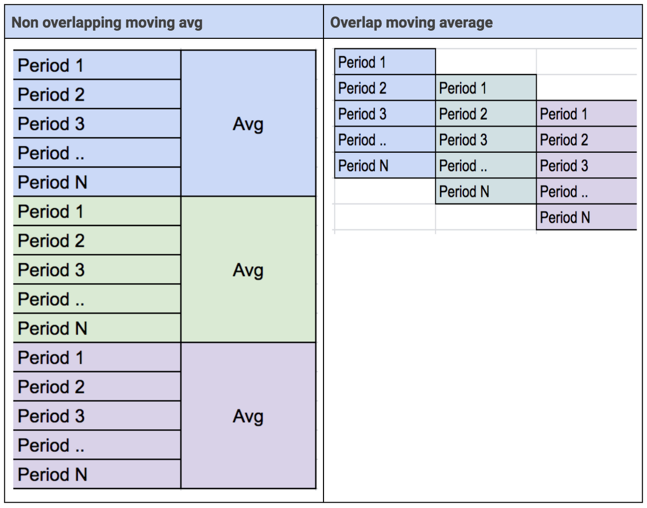

Here are a few simple functions to consider for feature engineering:


Model architecture and algorithms to use
Once you’ve built your feature detectors, the next step is to decide what algorithms you wish to try for the model-building phase.
Depending on your use case, you need to determine whether you should apply a:
Supervised or unsupervised learning approach
Classification or regression approach
Traditional ML or deep learning approach
Supervised learning
Use supervised learning if you have labeled your dataset with machinery failures. Traditional ML find patterns inside your dataset. Deep Learning can find patterns inside patterns or even hidden patterns.
Traditional machine learning versus deep learning
Traditional ML, or DNN models, work on individual data point values. Sometimes a data sequence will show failure signals such as spikes. To find such patterns, you need a model algorithm that can find patterns in a sequence. The Recurrent Neural Network (RNN) was designed in 1980 to solve this specific problem: the RNN has internal memory that helps it find patterns across a sequence, such as spikes.
Advanced deep learning models
RNN models were originally designed for language use cases, such as translation, speech, and natural language use cases. Sentences can be defined as mere sequences of words, and RNN models handle conext by remembering those word sequences.
Internet of Things (IoT) data also often contain sequences. When learning from sequential data it is natural to consider Hidden Markov Models and Recurrent Neural Networks (RNNs). Hidden Markov Models can predict state based on current state. On the other hand, RNN models are more useful when predicting the state based on all previous states, since a RNN can be unfolded in time backpropagating over t timesteps

In this sense, the RNN is generally effective for time-series data. However, RNN can have trouble remembering input that occurs long time ago in the sequence. That is, RNNs have difficulty maintaining long-term temporal dependencies. This is due to the gradient of the loss function decays exponentially with time.
While RNN models handle sequence well, they have limitations based on sequence length. The Long Short Term Memory (LSTM) is a variation of the RNN model architecture. A given LSTM model is capable of learning long-term dependencies in a sequence of data. If you have a sequence of IoT data and symptoms of failures are spread across sequence, then a LSTM model architecture can identify these patterns and build models to detect them.
Unsupervised algorithms
There are many occasions when you want to identify unusual behavior or patterns. The ability to identify anomalies is useful when you encounter expected patterns. You can monitor the health of system and trigger alerts when anomalous behavior is observed. There are a number of statistical and machine learning methods that can identify anomalies in a system.
Traditional machine learning versus deep learning
Autoencoders are a neural network-based method typically used to find anomalies in complex vectors. They use back-propagation and set the target values equal to input values. Using an autoencoder lets you create benchmarks or identify anomalies in complex vectors.
Metrics
The most important design decision (or question) in machine learning model building is: “What metric do you want to optimize for?” You should select a metric based on your primary business objective.
If your dataset has 99.5% good example and .5% failure. You can get a 99.5% accuracy simply by classifying each instance as good. Clearly, accuracy can’t be a suitable metric for scenarios in which you are trying to identify “rare failures”.
Here are metrics to consider as you work to answer business questions:
Metrics for binary classification
Precision
Precision will answer the following question: out of a set of equipment classified “will fail,” what fraction of the predictions were correct?
Precision = tp/(tp+fp)
Recall or sensitivity
Recall will answer the question: out of equipment that “actually failed” what fraction did the classifier pick up?
Recall, or Sensitivity = tp/(tp+fn)
Recall is also called sensitivity and measures the percentage of trials that a positive prediction holds true.
Accuracy
Accuracy refers to the degree of correctness for all trials. It is the ratio of correct predictions to (over) total examples.
Precision = tp+tn/(tp+tn +fp+ fn)
Accuracy is a good measure if the incidence of the multiple classes is balanced. But accuracy is not a good metric if you are trying to find failure for the case in which the total number of failures is very small.
F1 score
F1 score is the harmonic mean of Precision and Recall.
F1 = 2 *(precision*recall) /precision + recall)
True positive rate
TPrate refers to percentage of correctly classified failure instances.
TPrate = tp/(tp+fn)
TPrate is also called sensitivity or recall and represents the true positive rate.
True negative rate
TNrate refers to percentage of correctly classified normal instances.
TPrate = Tn/(Tn+Fp)
False positive rate
FPrate refers to percentage of incorrectly classified failure instances.
FPrate = Fp/(Fp+Tn)
False negative rate
FPrate refers to percentage of incorrectly classified normal instances.
FNrate = Fn/(Fn+Tp)
ROC (receiver operating characteristic) curve
An ROC curve shows how a given model’s predictions create different TP vs. FP rates when different decision thresholds are used.
As we lower the threshold, we are likely to have more false positives, but will also increase the number of true positives we find.


Metrics for multi-class classification
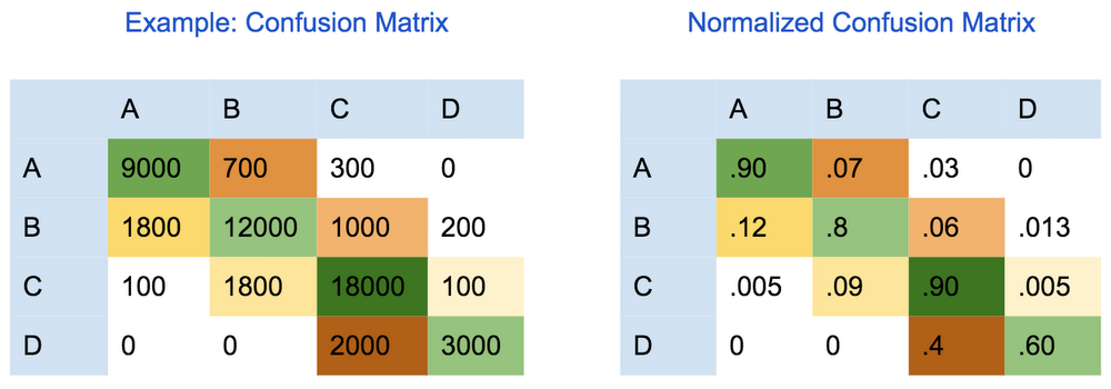
To evaluate the quality of a machine learning model for a multi-class classification model, you can use the “confusion (error) matrix”. In a confusion matrix, each row represents the count of instances for the true class and each column represents the number of instances obtained for the predicted class. Therefore, the diagonal cells represent the number of points for which the predicted label is equal to the true label. Similarly, off-diagonal elements are those that are mislabeled by the classifier.
Higher values in off-diagonal cells indicate incorrect predictions of the model. Error analysis should be done on such cells to understand how the model makes classification errors among the different classes.

Macro and micro averages for precision, recall, and accuracy
Precision, recall, and accuracy are important measures for binary classification. When dealing with multiple classes, there are typically two approaches to compute precision, recall and accuracy.
Micro-precision/recall: each example is assigned equal weight. In this method, the micro average will aggregate the contributions of all classes when calculating the average. That is, you sum up individual true positive (TP), false positive (FP), true negative (TN), and false negative (FN) values. Hence, all examples get equal weight in computing precision recall.
Macro-precision/recall: each class is assigned equal weight. In macro average precision or recall you compute precision and recall for each class and then take average.
Metrics for regression
To predict remaining useful life for equipment, you will typically use a regression metric.Common metrics are:
Mean absolute error
Mean Absolute Error (MAE) measures the difference between the predicted value and the actual value and gets average difference. You should use the absolute difference, sum it and then divide by the number of samples.
Root mean square error
Root Mean Square Error (RMSE) is similar to MAE, except that it penalizes large errors more. RMSE squares the differences between predicted and actual value, calculates the average difference, and then take the square root of that average difference.
Mean absolute percentage error
Mean Absolute Percentage Error (MAPE) measure the size of error as a percentage, so MAPE is easy to interpret. MAPE is better to use when actual values are not uniform and you can normalize values using percentages.
Conclusion
When building a machine learning model for predictive maintenance, it is important that you validate that your data has a pattern that shows equipment degradation with age or usage.
To start the predictive maintenance journey, first define use case as mentioned in Part I here. Decide on your definition of equipment failure. Then, ensure that you already have, or can generate a dataset that matches your use case. To validate that your dataset has the matching pattern to build your model, you should use simple data exploration techniques to determine whether your data includes degradation or failure patterns. Once you find evidence of a pattern, you are ready to build your model.
If the raw data does not reveal a degradation pattern, you should perform feature engineering and bring your data into a state (shape) that highlights machinery degradation. If you can see a degradation pattern during data exploration, it is highly likely that a machine learning model will work with great accuracy. In addition, deep learning-based techniques have the capability to find patterns that are not visible through data exploration techniques. You should consider using deep learning as it finds patterns inside patterns which traditional machine learning can’t find.
Very often raw data does not directly exhibit a pattern, but an implicit pattern exists in spikes or other sequence types. Deep Learning provides both RNN and LSTM modeling architectures that handle sequences well.
Once you have prepared your data, select algorithm to train your machine learning model. After the initial version of the model is built, focus on fine tuning model to achieve higher accuracy based on the metric you selected. It is important to select the right metric that aligns with use cases and business objectives specific to your team.
In our final installment, we’ll provide some useful examples of these types of models in action.
