Advanced Guide to Inception v3

This document discusses aspects of the Inception model and how they come together to make the model run efficiently on Cloud TPU. It is an advanced view of the guide to running Inception v3 on Cloud TPU. Specific changes to the model that led to significant improvements are discussed in more detail. This document supplements the Inception v3 tutorial.

Inception v3 TPU training runs match accuracy curves produced by GPU jobs of similar configuration. The model has been successfully trained on v2-8, v2-128, and v2-512 configurations. The model has attained greater than 78.1% accuracy in about 170 epochs.

The code samples shown in this document are meant to be illustrative, a high-level picture of what happens in the actual implementation. Working code can be found on GitHub.

Introduction

Inception v3 is an image recognition model that has been shown to attain greater than 78.1% accuracy on the ImageNet dataset. The model is the culmination of many ideas developed by multiple researchers over the years. It is based on the original paper: "Rethinking the Inception Architecture for Computer Vision" by Szegedy, et. al.

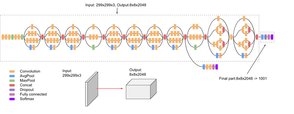
The model itself is made up of symmetric and asymmetric building blocks, including convolutions, average pooling, max pooling, concatenations, dropouts, and fully connected layers. Batch normalization is used extensively throughout the model and applied to activation inputs. Loss is computed using Softmax.

A high-level diagram of the model is shown in the following screenshot:

Estimator API

Warning: TPUEstimator is only available in TensorFlow 1.x. If you are writing a model with TensorFlow 2.x, use Keras instead.

The TPU version of Inception v3 is written using TPUEstimator, an API designed to facilitate development, so that you can focus on the models themselves rather than on the details of the underlying hardware. The API does most of the low-level grunge work necessary for running models on TPUs behind the scenes, while automating common functions, such as saving and restoring checkpoints.

The Estimator API enforces separation of model and input portions of the code. You define model_fn and input_fn functions, corresponding to the model definition and input pipeline. The following code shows the declaration of these functions:

def model_fn(features, labels, mode, params):
     …
  return tpu_estimator.TPUEstimatorSpec(mode=mode, loss=loss, train_op=train_op)

def input_fn(params):
    def parser(serialized_example):
          …
        return image, label

          …
   images, labels = dataset.make_one_shot_iterator().get_next()
   return images, labels

Two key functions provided by the API are train() and evaluate() used to train and evaluate as shown in the following code:

def main(unused_argv):
  …
  run_config = tpu_config.RunConfig(
      master=FLAGS.master,
      model_dir=FLAGS.model_dir,
      session_config=tf.ConfigProto(
          allow_soft_placement=True, log_device_placement=True),
      tpu_config=tpu_config.TPUConfig(FLAGS.iterations, FLAGS.num_shards),)

  estimator = tpu_estimator.TPUEstimator(
      model_fn=model_fn,
      use_tpu=FLAGS.use_tpu,
      train_batch_size=FLAGS.batch_size,
      eval_batch_size=FLAGS.batch_size,
      config=run_config)

  estimator.train(input_fn=input_fn, max_steps=FLAGS.train_steps)

  eval_results = inception_classifier.evaluate(
      input_fn=imagenet_eval.input_fn, steps=eval_steps)

ImageNet dataset

Before the model can be used to recognize images, it must be trained using a large set of labeled images. ImageNet is a common dataset to use.

ImageNet has over ten million URLs of labeled images. One million of the images also have bounding boxes specifying a more precise location for the labeled objects.

For this model, the ImageNet dataset is composed of 1,331,167 images which are split into training and evaluation datasets containing 1,281,167 and 50,000 images, respectively.

The training and evaluation datasets are kept separate intentionally. Only images from the training dataset are used to train the model and only images from the evaluation dataset are used to evaluate model accuracy.

The model expects images to be stored as TFRecords. For more information about how to convert images from raw JPEG files into TFRecords, see download_and_preprocess_imagenet.sh.

Input pipeline

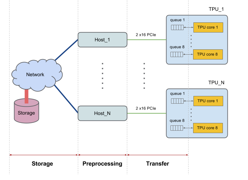
Each Cloud TPU device has 8 cores and is connected to a host (CPU). Larger slices have multiple hosts. Other larger configurations interact with multiple hosts. For example a v2-256 communicates with 16 hosts.

Hosts retrieve data from the file system or local memory, do whatever data preprocessing is required, and then transfer preprocessed data to the TPU cores. We consider these three phases of data handling done by the host individually and refer to the phases as: 1) Storage, 2) Preprocessing, 3) Transfer. A high-level picture of the diagram is shown in the following figure:

To yield good performance, the system should be balanced. If the host CPU takes longer than the TPU to complete the three data handling phases, then execution will be host-bound. Both cases are shown in the following diagram:

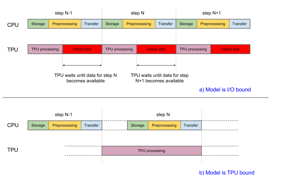
The current implementation of Inception v3 is at the edge of being input-bound. Images are retrieved from the file system, decoded, and then preprocessed. Different types of preprocessing stages are available, ranging from moderate to complex. If we use the most complex of preprocessing stages, the training pipeline will be preprocessing bound. You can attain accuracy greater than 78.1% using a moderately complex preprocessing stage that keeps the model TPU-bound.

The model uses tf.data.Dataset to handle input pipeline processing. For more information about how to optimize input pipelines, see the datasets performance guide.

Although you can define a function and pass it to the Estimator API, the class InputPipeline encapsulates all required features.

The Estimator API makes it straightforward to use this class. You pass it to the input_fn parameter of functions train() and evaluate(), as shown in the following code snippet:

def main(unused_argv):

          …

  inception_classifier = tpu_estimator.TPUEstimator(
      model_fn=inception_model_fn,
      use_tpu=FLAGS.use_tpu,
      config=run_config,
      params=params,
      train_batch_size=FLAGS.train_batch_size,
      eval_batch_size=eval_batch_size,
      batch_axis=(batch_axis, 0))

          …

  for cycle in range(FLAGS.train_steps // FLAGS.train_steps_per_eval):
    tf.logging.info('Starting training cycle %d.' % cycle)
    inception_classifier.train(
        input_fn=InputPipeline(True), steps=FLAGS.train_steps_per_eval)

    tf.logging.info('Starting evaluation cycle %d .' % cycle)
    eval_results = inception_classifier.evaluate(
        input_fn=InputPipeline(False), steps=eval_steps, hooks=eval_hooks)
    tf.logging.info('Evaluation results: %s' % eval_results)

The main elements of InputPipeline are shown in the following code snippet.

class InputPipeline(object):

  def __init__(self, is_training):
    self.is_training = is_training

  def __call__(self, params):
    # Storage
    file_pattern = os.path.join(
        FLAGS.data_dir, 'train-*' if self.is_training else 'validation-*')
    dataset = tf.data.Dataset.list_files(file_pattern)
    if self.is_training and FLAGS.initial_shuffle_buffer_size > 0:
      dataset = dataset.shuffle(
          buffer_size=FLAGS.initial_shuffle_buffer_size)
    if self.is_training:
      dataset = dataset.repeat()

    def prefetch_dataset(filename):
      dataset = tf.data.TFRecordDataset(
          filename, buffer_size=FLAGS.prefetch_dataset_buffer_size)
      return dataset

    dataset = dataset.apply(
        tf.contrib.data.parallel_interleave(
            prefetch_dataset,
            cycle_length=FLAGS.num_files_infeed,
            sloppy=True))
    if FLAGS.followup_shuffle_buffer_size > 0:
      dataset = dataset.shuffle(
          buffer_size=FLAGS.followup_shuffle_buffer_size)

    # Preprocessing
    dataset = dataset.map(
        self.dataset_parser,
        num_parallel_calls=FLAGS.num_parallel_calls)

    dataset = dataset.prefetch(batch_size)
    dataset = dataset.apply(
        tf.contrib.data.batch_and_drop_remainder(batch_size))
    dataset = dataset.prefetch(2)  # Prefetch overlaps in-feed with training
    images, labels = dataset.make_one_shot_iterator().get_next()

    # Transfer
    return images, labels

The storage section begins with the creation of a dataset and includes the reading of TFRecords from storage (using tf.data.TFRecordDataset). Special purpose functions repeat() and shuffle() are used as needed. Function tf.contrib.data.parallel_interleave() maps function prefetch_dataset() across its input to produce nested datasets, and outputs their elements interleaved. It gets elements from cycle_length nested datasets in parallel, which increases throughput. The sloppy argument relaxes the requirement that the outputs be produced in a deterministic order, and allows the implementation to skip over nested datasets whose elements are not readily available when requested.

The preprocessing section calls dataset.map(parser) which in turn calls the parser function where images are preprocessed. The details of the preprocessing stage are discussed in the next section.

The transfer section (at the end of the function) includes the line return images, labels. TPUEstimator takes the returned values and automatically transfers them to the device.

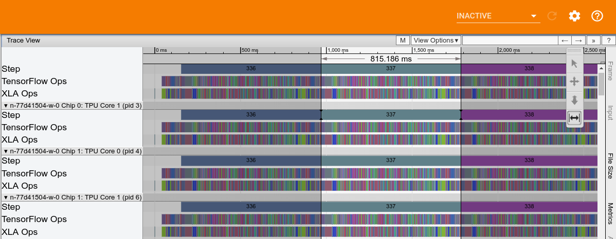
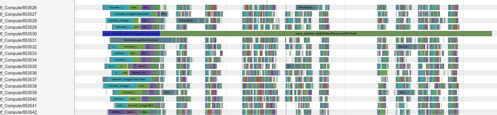
The following figure shows a sample Cloud TPU performance trace of Inception v3. TPU compute time, ignoring any in-feeding stalls, is approximately 815 msecs.

Host storage is written to the trace and shown in the following screenshot:

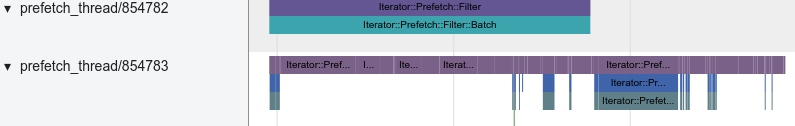
Host preprocessing, which includes image decoding and a series of image distortion functions is shown in the following screenshot:

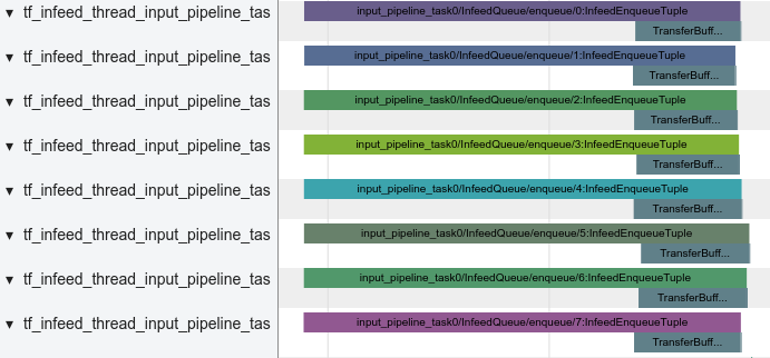
Host/TPU transfer is shown in the following screenshot:

Preprocessing Stage

Image preprocessing is a crucial part of the system and can influence the maximum accuracy that the model attains during training. At a minimum, images need to be decoded and resized to fit the model. For Inception, images need to be 299x299x3 pixels.

However, simply decoding and resizing are not enough to get good accuracy. The ImageNet training dataset contains 1,281,167 images. One pass over the set of training images is referred to as an epoch. During training, the model requires several passes through the training dataset to improve its image recognition capabilities. To train Inception v3 to sufficient accuracy, use between 140 and 200 epochs depending on the global batch size.

It is useful to continuously alter the images before feeding them to the model so that a particular image is slightly different at every epoch. How to best do this preprocessing of images is as much art as it is science. A well-designed preprocessing stage can significantly boost the recognition capabilities of a model. Too simple a preprocessing stage may create an artificial ceiling on the accuracy that the same model can attain during training.

Inception v3 offers options for the preprocessing stage, ranging from relatively simple and computationally inexpensive to fairly complex and computationally expensive. Two distinct flavors of such can be found in files vgg_preprocessing.py and inception_preprocessing.py.

File vgg_preprocessing.py defines a preprocessing stage that has been used successfully to train resnet to 75% accuracy, but yields suboptimal results when applied on Inception v3.

File inception_preprocessing.py contains a preprocessing stage that has been used to train Inception v3 with accuracies between 78.1 and 78.5% when run on TPUs.

Preprocessing differs depending on whether the model is undergoing training or being used for inference/evaluation.

At evaluation time, preprocessing is straightforward: crop a central region of the image and then resize it to the default 299x299 size. The following code snippet shows a preprocessing implementation:

def preprocess_for_eval(image, height, width, central_fraction=0.875):
  with tf.name_scope(scope, 'eval_image', [image, height, width]):
    if image.dtype != tf.float32:
      image = tf.image.convert_image_dtype(image, dtype=tf.float32)
    image = tf.image.central_crop(image, central_fraction=central_fraction)
    image = tf.expand_dims(image, 0)
    image = tf.image.resize_bilinear(image, [height, width], align_corners=False)
    image = tf.squeeze(image, [0])
    image = tf.subtract(image, 0.5)
    image = tf.multiply(image, 2.0)
    image.set_shape([height, width, 3])
    return image

During training, the cropping is randomized: a bounding box is chosen randomly to select a region of the image which is then resized. The resized image is then optionally flipped and its colors are distorted. The following code snippet shows an implementation of these operations:

def preprocess_for_train(image, height, width, bbox, fast_mode=True, scope=None):
  with tf.name_scope(scope, 'distort_image', [image, height, width, bbox]):
    if bbox is None:
      bbox = tf.constant([0.0, 0.0, 1.0, 1.0], dtype=tf.float32, shape=[1, 1, 4])
    if image.dtype != tf.float32:
      image = tf.image.convert_image_dtype(image, dtype=tf.float32)

    distorted_image, distorted_bbox = distorted_bounding_box_crop(image, bbox)
    distorted_image.set_shape([None, None, 3])

    num_resize_cases = 1 if fast_mode else 4
    distorted_image = apply_with_random_selector(
        distorted_image,
        lambda x, method: tf.image.resize_images(x, [height, width], method),
        num_cases=num_resize_cases)

    distorted_image = tf.image.random_flip_left_right(distorted_image)

    if FLAGS.use_fast_color_distort:
      distorted_image = distort_color_fast(distorted_image)
    else:
      num_distort_cases = 1 if fast_mode else 4
      distorted_image = apply_with_random_selector(
          distorted_image,
          lambda x, ordering: distort_color(x, ordering, fast_mode),
          num_cases=num_distort_cases)

    distorted_image = tf.subtract(distorted_image, 0.5)
    distorted_image = tf.multiply(distorted_image, 2.0)
    return distorted_image

Function distort_color is in charge of color alteration. It offers a fast mode where only brightness and saturation are modified. The full mode modifies brightness, saturation, and hue, in a random order.

def distort_color(image, color_ordering=0, fast_mode=True, scope=None):
  with tf.name_scope(scope, 'distort_color', [image]):
    if fast_mode:
      if color_ordering == 0:
        image = tf.image.random_brightness(image, max_delta=32. / 255.)
        image = tf.image.random_saturation(image, lower=0.5, upper=1.5)
      else:
        image = tf.image.random_saturation(image, lower=0.5, upper=1.5)
        image = tf.image.random_brightness(image, max_delta=32. / 255.)
    else:
      if color_ordering == 0:
        image = tf.image.random_brightness(image, max_delta=32. / 255.)
        image = tf.image.random_saturation(image, lower=0.5, upper=1.5)
        image = tf.image.random_hue(image, max_delta=0.2)
        image = tf.image.random_contrast(image, lower=0.5, upper=1.5)
      elif color_ordering == 1:
        image = tf.image.random_saturation(image, lower=0.5, upper=1.5)
        image = tf.image.random_brightness(image, max_delta=32. / 255.)
        image = tf.image.random_contrast(image, lower=0.5, upper=1.5)
        image = tf.image.random_hue(image, max_delta=0.2)
      elif color_ordering == 2:
        image = tf.image.random_contrast(image, lower=0.5, upper=1.5)
        image = tf.image.random_hue(image, max_delta=0.2)
        image = tf.image.random_brightness(image, max_delta=32. / 255.)
        image = tf.image.random_saturation(image, lower=0.5, upper=1.5)
      elif color_ordering == 3:
        image = tf.image.random_hue(image, max_delta=0.2)
        image = tf.image.random_saturation(image, lower=0.5, upper=1.5)
        image = tf.image.random_contrast(image, lower=0.5, upper=1.5)
        image = tf.image.random_brightness(image, max_delta=32. / 255.)

    return tf.clip_by_value(image, 0.0, 1.0)

Function distort_color is computationally expensive, partly due to the nonlinear RGB to HSV and HSV to RGB conversions that are required in order to access hue and saturation. Both fast and full modes require these conversions and although fast mode is less computationally expensive, it still pushes the model to the CPU-compute-bound region, when enabled.

As an alternative, a new function distort_color_fast has been added to the list of options. This function maps the image from RGB to YCrCb using the JPEG conversion scheme and randomly alters brightness and the Cr/Cb chromas before mapping back to RGB. The following code snippet shows an implementation of this function:

def distort_color_fast(image, scope=None):
  with tf.name_scope(scope, 'distort_color', [image]):
    br_delta = random_ops.random_uniform([], -32./255., 32./255., seed=None)
    cb_factor = random_ops.random_uniform(
        [], -FLAGS.cb_distortion_range, FLAGS.cb_distortion_range, seed=None)
    cr_factor = random_ops.random_uniform(
        [], -FLAGS.cr_distortion_range, FLAGS.cr_distortion_range, seed=None)

    channels = tf.split(axis=2, num_or_size_splits=3, value=image)
    red_offset = 1.402 * cr_factor + br_delta
    green_offset = -0.344136 * cb_factor - 0.714136 * cr_factor + br_delta
    blue_offset = 1.772 * cb_factor + br_delta
    channels[0] += red_offset
    channels[1] += green_offset
    channels[2] += blue_offset
    image = tf.concat(axis=2, values=channels)
    image = tf.clip_by_value(image, 0., 1.)
    return image

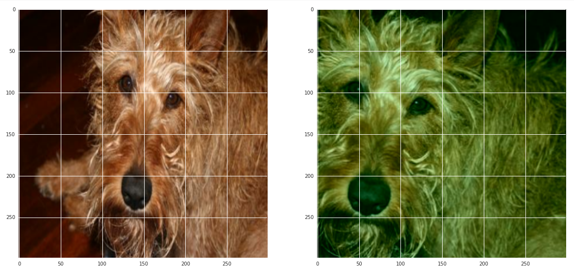
Here's a sample image that has undergone preprocessing. A randomly chosen region of the image has been selected and colors altered using the distort_color_fast function.

Function distort_color_fast is computationally efficient and still allows training to be TPU execution time bound. In addition, it has been used to train the Inception v3 model to an accuracy greater than 78.1% using batch sizes in the 1,024-16,384 range.

Optimizer

The current model showcases three flavors of optimizers: SGD, momentum, and RMSProp.

Stochastic gradient descent (SGD) is the simplest update: the weights are nudged in the negative gradient direction. Despite its simplicity, good results can still be obtained on some models. The updates dynamics can be written as:

$$w_{k+1}=w_k-\alpha∇f(w_k)$$

Momentum is a popular optimizer that frequently leads to faster convergence than SGD. This optimizer updates weights much like SGD but also adds a component in the direction of the previous update. The following equations describe the updates performed by the momentum optimizer:

$$z_{k+1}=\beta z_k+∇f(w_k)$$

$$w_{k+1}=w_k-\alpha z_{k+1}$$

which can be written as:

$$w_{k+1}=w_k-\alpha ∇f(w_k)+\beta \left(w_k-w_{k-1}\right)$$

The last term is the component in the direction of the previous update.

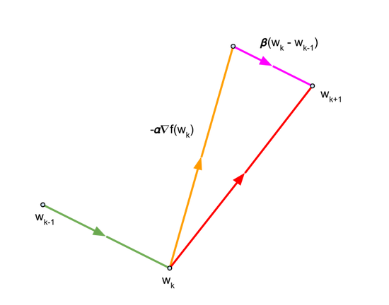
For the momentum \({\beta}\), we use the value of 0.9.

RMSprop is a popular optimizer first proposed by Geoff Hinton in one of his lectures. The following equations describe how the optimizer works:

$$g_{k+1}^{-2} = \alpha g_{k}^{-2} + (1-\alpha) g_{k}^2$$ $$w_{k+1}=\beta w_k + \frac{\eta}{\sqrt {g_{k+1^{\mathbf{+{\epsilon}}}}^{-2}}} ∇f(w_k)$$

For Inception v3, tests show RMSProp giving the best results in terms of maximum accuracy and time to attain it, with momentum a close second. Thus RMSprop is set as the default optimizer. The parameters used are: decay \({\alpha}\) = 0.9, momentum \({\beta}\) = 0.9, and \({\epsilon}\) = 1.0.

The following code snippet shows how to set these parameters:

if FLAGS.optimizer == 'sgd':
  tf.logging.info('Using SGD optimizer')
  optimizer = tf.train.GradientDescentOptimizer(
      learning_rate=learning_rate)
elif FLAGS.optimizer == 'momentum':
  tf.logging.info('Using Momentum optimizer')
  optimizer = tf.train.MomentumOptimizer(
      learning_rate=learning_rate, momentum=0.9)
elif FLAGS.optimizer == 'RMS':
  tf.logging.info('Using RMS optimizer')
  optimizer = tf.train.RMSPropOptimizer(
      learning_rate,
      RMSPROP_DECAY,
      momentum=RMSPROP_MOMENTUM,
      epsilon=RMSPROP_EPSILON)
else:
  tf.logging.fatal('Unknown optimizer:', FLAGS.optimizer)

When running on TPUs and using the Estimator API, the optimizer needs to be wrapped in a CrossShardOptimizer function in order to ensure synchronization among the replicas (along with any necessary cross communication). The following code snippet shows how the Inception v3 model wraps the optimizer:

if FLAGS.use_tpu:
    optimizer = tpu_optimizer.CrossShardOptimizer(optimizer)

update_ops = tf.get_collection(tf.GraphKeys.UPDATE_OPS)
with tf.control_dependencies(update_ops):
  train_op = optimizer.minimize(loss, global_step=global_step)

Exponential moving average

While training, the trainable parameters are updated during backpropagation according to the optimizer's update rules. The equations describing these rules were discussed in the previous section and repeated here for convenience:

$${\theta_{k+1}} = {\theta_k}-{\alpha ∇f(\theta_k)} \qquad(SGD)$$

$${\theta_{k+1}}={\theta_k}-{\alpha z_{k+1}} \qquad(momentum)$$

$${\theta_{k+1}}= {\beta \theta_k}+\frac{\eta}{\sqrt {g_{k+1^{\mathbf+{\epsilon}}}}^{-2}} ∇f(\theta_k) \qquad(RMSprop)$$

Exponential moving average (also known as exponential smoothing) is an optional post-processing step that is applied to the updated weights and can sometimes lead to noticeable improvements in performance. TensorFlow provides the function tf.train.ExponentialMovingAverage that computes the ema \({\hat{\theta}}\) of weight \({\theta}\) using the formula:

$${\hat{\theta_t}}={\alpha {\hat{\theta}{_{t-1}}}}+{(1-\alpha)}{\theta_t}$$

where \({\alpha}\) is a decay factor (close to 1.0). In the Inception v3 model, \({\alpha}\) is set to 0.995.

Even though this calculation is an Infinite Impulse Response (IIR) filter, the decay factor establishes an effective window where most of the energy (or relevant samples) resides, as shown in the following diagram:

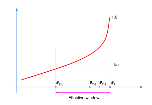
We can rewrite the filter equation, as follows:

$${\hat{\theta}_{t+T+1}}={\alpha(1-\alpha)}({\theta_{t+T}}+{\alpha \theta_{t+T-1}}+...+{\alpha^{t+T}}{\theta_0})$$

where we used \({\hat\theta_{-1}}=0\).

The \({\alpha}^k\) values decay with increasing k, so only a subset of the samples will have a sizable influence on \(\hat{\theta}_{t+T+1}\). The rule of thumb for the decay factor value is: \(\frac {1} {1-\alpha}\), which corresponds to \({\alpha}\) = 200 for =0.995.

We first get a collection of trainable variables and then use the apply() method to create shadow variables for each trained variable. The following code snippet shows the Inception v3 model implementation:

update_ops = tf.get_collection(tf.GraphKeys.UPDATE_OPS)
with tf.control_dependencies(update_ops):
  train_op = optimizer.minimize(loss, global_step=global_step)

if FLAGS.moving_average:
  ema = tf.train.ExponentialMovingAverage(
      decay=MOVING_AVERAGE_DECAY, num_updates=global_step)
  variables_to_average = (tf.trainable_variables() +
                          tf.moving_average_variables())
  with tf.control_dependencies([train_op]), tf.name_scope('moving_average'):
    train_op = ema.apply(variables_to_average)

We'd like to use the ema variables during evaluation. We define class LoadEMAHook that applies method variables_to_restore() to the checkpoint file to evaluate using the shadow variable names:

class LoadEMAHook(tf.train.SessionRunHook):
  def __init__(self, model_dir):
    super(LoadEMAHook, self).__init__()
    self._model_dir = model_dir

  def begin(self):
    ema = tf.train.ExponentialMovingAverage(MOVING_AVERAGE_DECAY)
    variables_to_restore = ema.variables_to_restore()
    self._load_ema = tf.contrib.framework.assign_from_checkpoint_fn(
        tf.train.latest_checkpoint(self._model_dir), variables_to_restore)

  def after_create_session(self, sess, coord):
    tf.logging.info('Reloading EMA...')
    self._load_ema(sess)

The hooks function is passed to evaluate() as shown in the following code snippet:

if FLAGS.moving_average:
    eval_hooks = [LoadEMAHook(FLAGS.model_dir)]
else:
    eval_hooks = []

    …

eval_results = inception_classifier.evaluate(
    input_fn=InputPipeline(False), steps=eval_steps, hooks=eval_hooks)

Batch normalization

Batch normalization is a widely used technique for normalizing input features on models that can lead to substantial reduction in convergence time. It is one of the more popular and useful algorithmic improvements in machine learning of recent years and is used across a wide range of models, including Inception v3.

Activation inputs are normalized by subtracting the mean and dividing by the standard deviation. To keep things balanced in the presence of back propagation, two trainable parameters are introduced in every layer. Normalized outputs \({\hat{x}}\) undergo a subsequent operation \({\gamma\hat{x}}+\beta\), where \({\gamma}\) and \({\beta}\) are a sort of standard deviation and mean learned by the model itself.

The full set of equations is in the paper and is repeated here for convenience:

Input: Values of x over a mini-batch: \(\Phi=\) { \({x_{1..m}\\} \) } Parameters to be learned: \({\gamma}\),\({\beta}\)

Output: { \({y_i}=BN_{\gamma,\beta}{(x_i)}\) }

\[{\mu_\phi} \leftarrow {\frac{1}{m}}{\sum_{i=1}^m}x_i \qquad \mathsf(mini-batch\ mean)\]

\[{\sigma_\phi}^2 \leftarrow {\frac{1}{m}}{\sum_{i=1}^m} {(x_i - {\mu_\phi})^2} \qquad \mathbf(mini-batch\ variance)\]

\[{\hat{x_i}} \leftarrow {\frac{x_i-{\mu_\phi}}{\sqrt {\sigma^2_\phi}+{\epsilon}}}\qquad \mathbf(normalize)\]

\[{y_i}\leftarrow {\gamma \hat{x_i}} + \beta \equiv BN_{\gamma,\beta}{(x_i)}\qquad \mathbf(scale \ and \ shift)\]

Normalization happens during training, but come evaluation time, we'd like the model to behave in a deterministic fashion: the classification result of an image should depend solely on the input image and not the set of images that are being fed to the model. Thus, we need to fix \({\mu}\) and \({\sigma}^2\) and use values that represent the image population statistics.

The model computes moving averages of the mean and variance over the minibatches:

\[{\hat\mu_i} = {\alpha \hat\mu_{t-1}}+{(1-\alpha)\mu_t}\]

\[{\hat\sigma_t}^2 = {\alpha{\hat\sigma^2_{t-1}}} + {(1-\alpha) {\sigma_t}^2}\]

In the specific case of Inception v3, a sensible decay factor had been obtained (using hyperparameter tuning) for use in GPUs. We would like to use this value on TPUs as well, but in order to do that, we need to make some adjustments.

Batch normalization moving mean and variance are both calculated using a loss pass filter, as shown in the following equation (here, \({y_t}\) represents moving mean or variance):

\[{y_t}={\alpha y_{t-1}}+{(1-\alpha)}{x_t} \]

(1)

In an 8x1 GPU (synchronous) job, each replica reads the current moving mean and updates it. The current replica must write the new moving variable before the next replica can read it.

When there are 8 replicas, the set of operations for an ensemble update is as follows:

\[{y_t}={\alpha y_{t-1}}+{(1-\alpha)}{x_t} \]

\[{y_{t+1}}={\alpha y_{t}}+{(1-\alpha)}{x_{t+1}} \]

\[{y_{t+2}}={\alpha y_{t+1}}+{(1-\alpha)}{x_{t+2}} \]

\[{y_{t+3}}={\alpha y_{t+2}}+{(1-\alpha)}{x_{t+3}} \]

\[{y_{t+4}}={\alpha y_{t+3}}+{(1-\alpha)}{x_{t+4}} \]

\[{y_{t+5}}={\alpha y_{t+4}}+{(1-\alpha)}{x_{t+5}} \]

\[{y_{t+6}}={\alpha y_{t+5}}+{(1-\alpha)}{x_{t+6}} \]

\[{y_{t+7}}={\alpha y_{t+6}}+{(1-\alpha)}{x_{t+7}} \]

This set of 8 sequential updates can be written as:

\[{y_{t+7}}={\alpha^8y_{t-1}}+(1-\alpha){\sum_{k=0}^7} {\alpha^{7-k}}{x_{t+k}}\]

(2)

In the current moving moment calculation implementation on TPUs, each shard performs calculations independently and there is no cross-shard communication. Batches are distributed to every shard and each of them processes 1/8th of the total number of batches (when there are 8 shards).

Although each shard computes the moving moments (that is, mean and variance), only the results from shard 0 are communicated back to the host CPU. So, effectively, only one replica is doing the moving mean/variance update:

\[{z_t}={\beta {z_{t-1}}}+{(1-\beta)u_t}\]

(3)

and this update happens at 1/8th the rate of its sequential counterpart. In order to compare GPU and TPU update equations, we need to align the respective timescales. Specifically, the set of operations that make up a set of 8 sequential updates on the GPU should be compared against a single update on the TPU as illustrated in the following diagram:

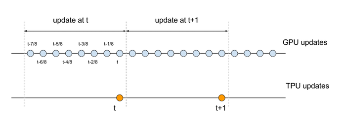
Let us show the equations with the modified time indexes:

\[{y_t}={\alpha^8y_{t-1}}+(1-\alpha){\sum_{k=0}^7} {\alpha^{7-k}}{x_{t-k/8}} \qquad \mathsf(GPU)\]

\[{z_t}={\beta {z_{t-1}}}+{(1-\beta)u_t}\qquad \mathsf(TPU) \]

If we make the assumption that 8 mini batches (normalized across all relevant dimensions) yield similar values within the GPU 8-minibatch sequential update, then we can approximate these equations as follows:

\[{y_t}={\alpha^8y_{t-1}}+(1-\alpha){\sum_{k=0}^7} {\alpha^{7-k}}{\hat{x_t}}={\alpha^8y_{t-1}+(1-\alpha^8){\hat{x_t}}} \qquad \mathsf(GPU)\]

\[{z_t}={\beta {z_{t-1}}}+{(1-\beta)u_t}\qquad \mathsf(TPU) \]

To match the effect of a given decay factor on the GPU, we modify the decay factor on the TPU accordingly. Specifically, we set \({\beta}\)=\({\alpha}^8\).

For Inception v3, the decay value used in the GPU is \({\alpha}\)=0.9997, which translates to a TPU decay value of \({\beta}\)=0.9976.

Learning rate adaptation

As batch sizes become larger, training becomes more difficult. Different techniques continue to be proposed to allow efficient training for large batch sizes (see here, here, and here, for example).

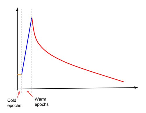
One of these techniques is increasing the learning rate gradually (also called ramp-up). Ramp-up was used to train the model to greater than 78.1% accuracy for batch sizes ranging from 4,096 to 16,384. For Inception v3, the learning rate is first set to about 10% of what would normally be the starting learning rate. The learning rate remains constant at this low value for a specified (small) number of 'cold epochs', and then begins a linear increase for a specified number of 'warm-up epochs'. At the end the 'warm-up epochs', the learning rate intersects with the normal exponential decay learning. This is illustrated in the following diagram.

The following code snippet shows how to do this:

initial_learning_rate = FLAGS.learning_rate * FLAGS.train_batch_size / 256
if FLAGS.use_learning_rate_warmup:
  warmup_decay = FLAGS.learning_rate_decay**(
    (FLAGS.warmup_epochs + FLAGS.cold_epochs) /
    FLAGS.learning_rate_decay_epochs)
  adj_initial_learning_rate = initial_learning_rate * warmup_decay

final_learning_rate = 0.0001 * initial_learning_rate

train_op = None
if training_active:
  batches_per_epoch = _NUM_TRAIN_IMAGES / FLAGS.train_batch_size
  global_step = tf.train.get_or_create_global_step()
  current_epoch = tf.cast(
    (tf.cast(global_step, tf.float32) / batches_per_epoch), tf.int32)

  learning_rate = tf.train.exponential_decay(
    learning_rate=initial_learning_rate,
    global_step=global_step,
    decay_steps=int(FLAGS.learning_rate_decay_epochs * batches_per_epoch),
    decay_rate=FLAGS.learning_rate_decay,
    staircase=True)

  if FLAGS.use_learning_rate_warmup:
    wlr = 0.1 * adj_initial_learning_rate
    wlr_height = tf.cast(
      0.9 * adj_initial_learning_rate /
      (FLAGS.warmup_epochs + FLAGS.learning_rate_decay_epochs - 1),
      tf.float32)
    epoch_offset = tf.cast(FLAGS.cold_epochs - 1, tf.int32)
    exp_decay_start = (FLAGS.warmup_epochs + FLAGS.cold_epochs +
                   FLAGS.learning_rate_decay_epochs)
    lin_inc_lr = tf.add(
      wlr, tf.multiply(
        tf.cast(tf.subtract(current_epoch, epoch_offset), tf.float32),
        wlr_height))
    learning_rate = tf.where(
      tf.greater_equal(current_epoch, FLAGS.cold_epochs),
      (tf.where(tf.greater_equal(current_epoch, exp_decay_start),
              learning_rate, lin_inc_lr)),
       wlr)

  # Set a minimum boundary for the learning rate.
  learning_rate = tf.maximum(
      learning_rate, final_learning_rate, name='learning_rate')