Query execution plans

PostgreSQL interface note: The examples in this topic are intended for GoogleSQL-dialect databases.

Overview

This page provides concepts about query execution plans and how they are used by Spanner to perform queries in a distributed environment. To learn how to retrieve an execution plan for a specific query using the Google Cloud console, see Understand how Spanner executes queries. You can also view sampled historic query plans and compare the performance of a query over time for certain queries. To learn more, see Sampled query plans.

Spanner uses declarative SQL statements to query its databases. SQL statements define what the user wants without specifying how to obtain the results. A query execution plan is the set of steps for how the results are obtained. For a given SQL statement, there may be multiple ways to obtain the results. The Spanner query optimizer evaluates different execution plans and chooses the one it considers to be most efficient. Spanner then uses the execution plan to retrieve the results.

Conceptually, an execution plan is a tree of relational operators. Each operator reads rows from its input(s) and produces output rows. The result of the operator at the root of the execution is returned as the result of the SQL query.

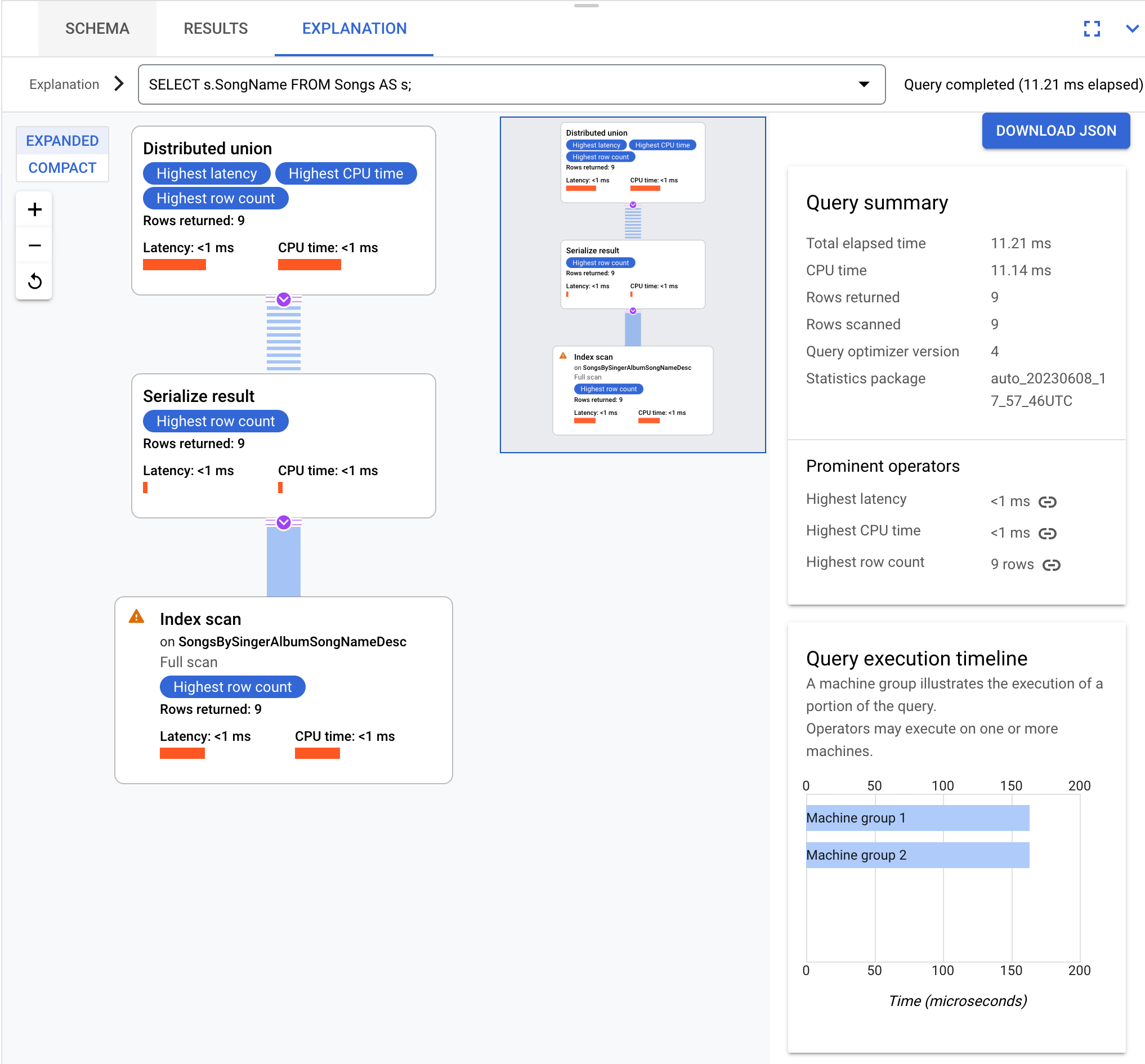
As an example, this query:

SELECT s.SongName FROM Songs AS s;

results in a query execution plan that can be visualized as:

The queries and execution plans on this page are based on the following database schema:

CREATE TABLE Singers (
  SingerId   INT64 NOT NULL,
  FirstName  STRING(1024),
  LastName   STRING(1024),
  SingerInfo BYTES(MAX),
  BirthDate  DATE
) PRIMARY KEY(SingerId);

CREATE INDEX SingersByFirstLastName ON Singers(FirstName, LastName);

CREATE TABLE Albums (
  SingerId        INT64 NOT NULL,
  AlbumId         INT64 NOT NULL,
  AlbumTitle      STRING(MAX),
  MarketingBudget INT64
) PRIMARY KEY(SingerId, AlbumId),
  INTERLEAVE IN PARENT Singers ON DELETE CASCADE;

CREATE INDEX AlbumsByAlbumTitle ON Albums(AlbumTitle);

CREATE INDEX AlbumsByAlbumTitle2 ON Albums(AlbumTitle) STORING (MarketingBudget);

CREATE TABLE Songs (
  SingerId  INT64 NOT NULL,
  AlbumId   INT64 NOT NULL,
  TrackId   INT64 NOT NULL,
  SongName  STRING(MAX),
  Duration  INT64,
  SongGenre STRING(25)
) PRIMARY KEY(SingerId, AlbumId, TrackId),
  INTERLEAVE IN PARENT Albums ON DELETE CASCADE;

CREATE INDEX SongsBySingerAlbumSongNameDesc ON Songs(SingerId, AlbumId, SongName DESC), INTERLEAVE IN Albums;

CREATE INDEX SongsBySongName ON Songs(SongName);

CREATE TABLE Concerts (
  VenueId      INT64 NOT NULL,
  SingerId     INT64 NOT NULL,
  ConcertDate  DATE NOT NULL,
  BeginTime    TIMESTAMP,
  EndTime      TIMESTAMP,
  TicketPrices ARRAY<INT64>
) PRIMARY KEY(VenueId, SingerId, ConcertDate);

You can use the following Data Manipulation Language (DML) statements to add data to these tables:

INSERT INTO Singers (SingerId, FirstName, LastName, BirthDate)
VALUES (1, "Marc", "Richards", "1970-09-03"),
       (2, "Catalina", "Smith", "1990-08-17"),
       (3, "Alice", "Trentor", "1991-10-02"),
       (4, "Lea", "Martin", "1991-11-09"),
       (5, "David", "Lomond", "1977-01-29");

INSERT INTO Albums (SingerId, AlbumId, AlbumTitle)
VALUES (1, 1, "Total Junk"),
       (1, 2, "Go, Go, Go"),
       (2, 1, "Green"),
       (2, 2, "Forever Hold Your Peace"),
       (2, 3, "Terrified"),
       (3, 1, "Nothing To Do With Me"),
       (4, 1, "Play");

INSERT INTO Songs (SingerId, AlbumId, TrackId, SongName, Duration, SongGenre)
VALUES (2, 1, 1, "Let's Get Back Together", 182, "COUNTRY"),
       (2, 1, 2, "Starting Again", 156, "ROCK"),
       (2, 1, 3, "I Knew You Were Magic", 294, "BLUES"),
       (2, 1, 4, "42", 185, "CLASSICAL"),
       (2, 1, 5, "Blue", 238, "BLUES"),
       (2, 1, 6, "Nothing Is The Same", 303, "BLUES"),
       (2, 1, 7, "The Second Time", 255, "ROCK"),
       (2, 3, 1, "Fight Story", 194, "ROCK"),
       (3, 1, 1, "Not About The Guitar", 278, "BLUES");

Note: You can run queries and retrieve execution plans even if the tables have no data.

Obtaining efficient execution plans is challenging because Spanner divides data into splits. Splits can move independently from each other and get assigned to different servers, which could be in different physical locations. To evaluate execution plans over the distributed data, Spanner uses execution based on:

• local execution of subplans in servers that contain the data
• orchestration and aggregation of multiple remote executions with aggressive distribution pruning

Spanner uses the primitive operator distributed union, along with its variants distributed cross apply and distributed outer apply, to enable this model.

Sampled query plans

Spanner sampled query plans allow you to view samples of historic query plans and compare the performance of a query over time. Not all queries have sampled query plans available. Only queries that consume higher CPU might be sampled. The data retention for Spanner query plan samples is 30 days. You can find query plan samples on the Query insights page of the Google Cloud console. For instructions, see View sampled query plans.

The anatomy of a sampled query plan is the same as a regular query execution plan. For more information on how to understand visual plans and use them to debug your queries, see A tour of the query plan visualizer.

Common use cases for sampled query plans:

Some common use cases for sampled query plans include:

• Observe query plan changes due to schema changes (for example, adding or removing an index).
• Observe query plan changes due to an optimizer version update.
• Observe query plan changes due to new optimizer statistics, which are collected every three days automatically or performed manually using the ANALYZE command.

If the performance of a query shows significant difference over time or if you want to improve the performance of a query, see SQL best practices to construct optimized query statements that help Spanner find efficient execution plans.

Life of a query

A SQL query in Spanner is first compiled into an execution plan, then it is sent to an initial root server for execution. The root server is chosen so as to minimize the number of hops to reach the data being queried. The root server then:

• initiates remote execution of subplans (if necessary)
• waits for results from the remote executions
• handles any remaining local execution steps such as aggregating results
• returns results for the query

Remote servers that receive a subplan act as a "root" server for their subplan, following the same model as the topmost root server. The result is a tree of remote executions. Conceptually, query execution flows from top to bottom, and query results are returned from bottom to top.The following diagram shows this pattern:

The following examples illustrate this pattern in more detail.

Aggregate queries

An aggregate query implements GROUP BY queries.

For example, using this query:

SELECT s.SingerId, COUNT(*) AS SongCount
FROM Songs AS s
WHERE s.SingerId < 100
GROUP BY s.SingerId;

These are the results:

+----------+-----------+
| SingerId | SongCount |
+----------+-----------+
|        3 |         1 |
|        2 |         8 |
+----------+-----------+

Conceptually, this is the execution plan:

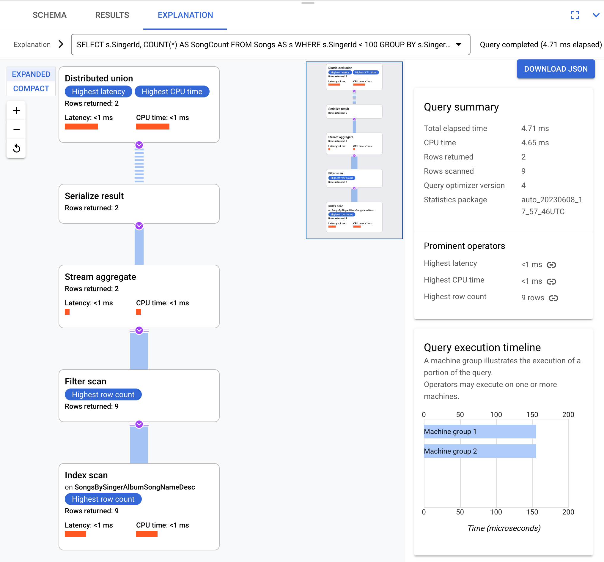
Spanner sends the execution plan to a root server that coordinates the query execution and performs the remote distribution of subplans.

This execution plan starts with a distributed union, which distributes subplans to remote servers whose splits satisfy SingerId < 100. After the scan on individual splits completes, the stream aggregate operator aggregates rows to get the counts for each SingerId. The serialize result operator then serializes the result. Finally, the distributed union combines all results together and returns the query results.

You can learn more about aggregates at aggregate operator.

Co-located join queries

Interleaved tables are physically stored with their rows of related tables co-located. A co-located join is a join between interleaved tables. Co-located joins can offer performance benefits over joins that require indexes or back joins.

For example, using this query:

SELECT al.AlbumTitle, so.SongName
FROM Albums AS al, Songs AS so
WHERE al.SingerId = so.SingerId AND al.AlbumId = so.AlbumId;

(This query assumes that Songs is interleaved in Albums.)

These are the results:

+-----------------------+--------------------------+
| AlbumTitle            | SongName                 |
+-----------------------+--------------------------+
| Nothing To Do With Me | Not About The Guitar     |
| Green                 | The Second Time          |
| Green                 | Starting Again           |
| Green                 | Nothing Is The Same      |
| Green                 | Let's Get Back Together  |
| Green                 | I Knew You Were Magic    |
| Green                 | Blue                     |
| Green                 | 42                       |
| Terrified             | Fight Story              |
+-----------------------+--------------------------+

This is the execution plan:

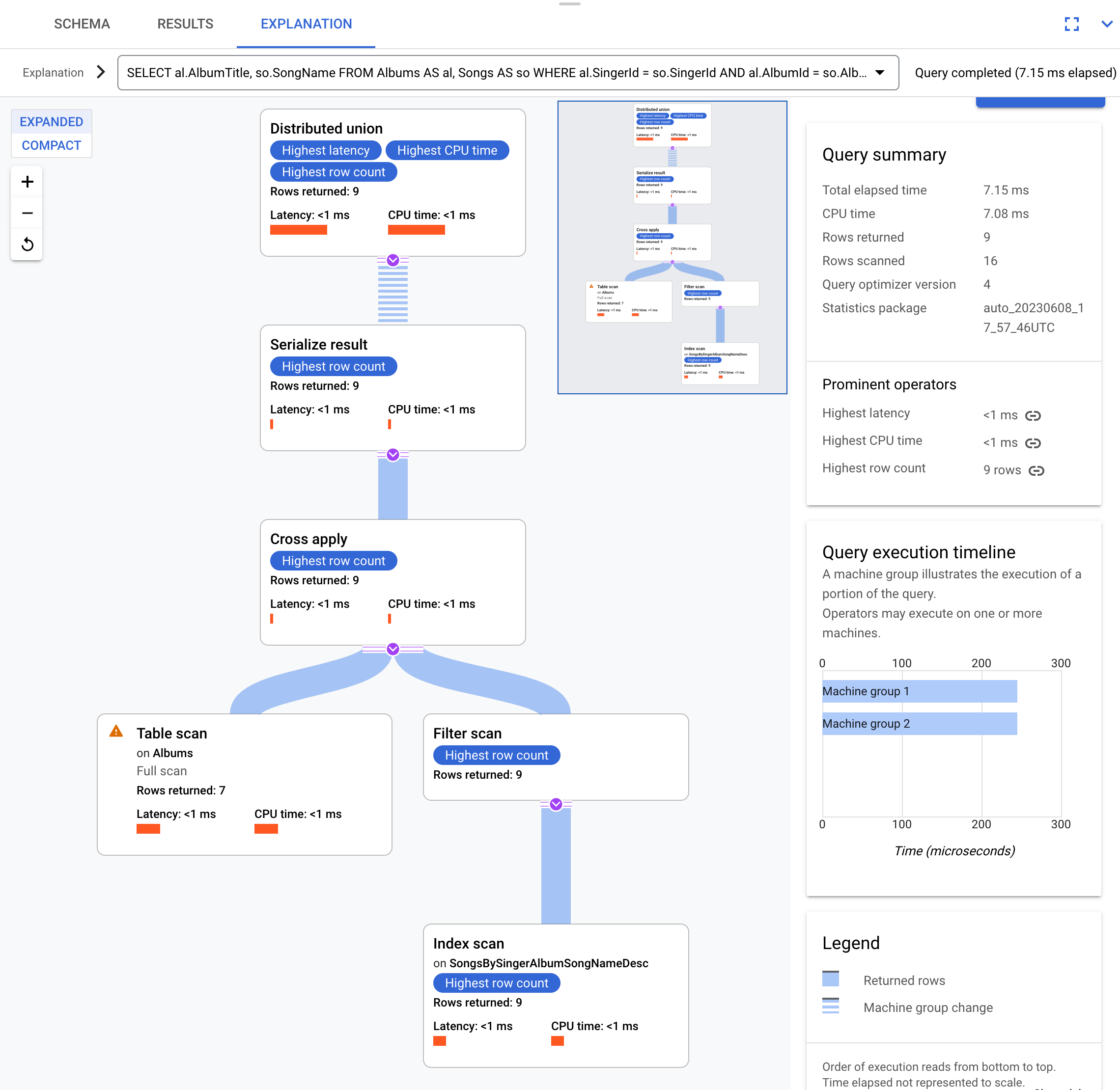
This execution plan starts with a distributed union, which distributes subplans to remote servers that have splits of the table Albums. Because Songs is an interleaved table of Albums, each remote server is able to execute the entire subplan on each remote server without requiring a join to a different server.

The subplans contain a cross apply. Each cross apply performs a table scan on table Albums to retrieve SingerId, AlbumId, and AlbumTitle. The cross apply then maps output from the table scan to output from an index scan on index SongsBySingerAlbumSongNameDesc, subject to a filter of the SingerId in the index matching the SingerId from the table scan output. Each cross apply sends its results to a serialize result operator which serializes the AlbumTitle and SongName data and returns results to the local distributed unions. The distributed union aggregates results from the local distributed unions and returns them as the query result.

Index and back join queries

The example above used a join on two tables, one interleaved in the other. Execution plans are more complex and less efficient when two tables, or a table and an index, are not interleaved.

Consider an index created with the following command:

CREATE INDEX SongsBySongName ON Songs(SongName)

Use this index in this query:

SELECT s.SongName, s.Duration
FROM Songs@{force_index=SongsBySongName} AS s
WHERE STARTS_WITH(s.SongName, "B");

These are the results:

+----------+----------+
| SongName | Duration |
+----------+----------+
| Blue     |      238 |
+----------+----------+

This is the execution plan:

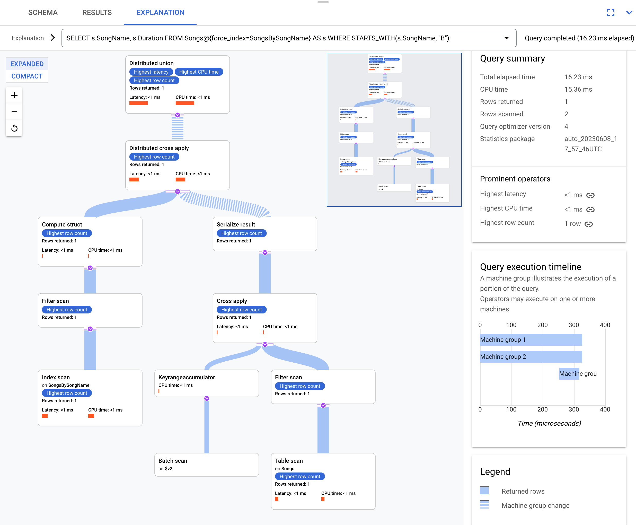
The resulting execution plan is complicated because the index SongsBySongName does not contain column Duration. To obtain the Duration value, Spanner needs to back join the indexed results to the table Songs. This is a join but it is not co-located because the Songs table and the global index SongsBySongName are not interleaved. The resulting execution plan is more complex than the co-located join example because Spanner performs optimizations to speed up the execution if data isn't co-located.

The top operator is a distributed cross apply. This input side of this operator are batches of rows from the index SongsBySongName that satisfy the predicate STARTS_WITH(s.SongName, "B"). The distributed cross apply then maps these batches to remote servers whose splits contain the Duration data. The remote servers use a table scan to retrieve the Duration column. The table scan uses the filter Condition:($Songs_key_TrackId' = $batched_Songs_key_TrackId), which joins TrackId from the Songs table to TrackId of the rows that were batched from the index SongsBySongName.

The results are aggregated into the final query answer. In turn, the input side of the distributed cross apply contains a distributed union/local distributed union pair to evaluate rows from the index that satisfy the STARTS_WITH predicate.

Consider a slightly different query that doesn't select the s.Duration column:

SELECT s.SongName
FROM Songs@{force_index=SongsBySongName} AS s
WHERE STARTS_WITH(s.SongName, "B");

This query is able to fully leverage the index as shown in this execution plan:

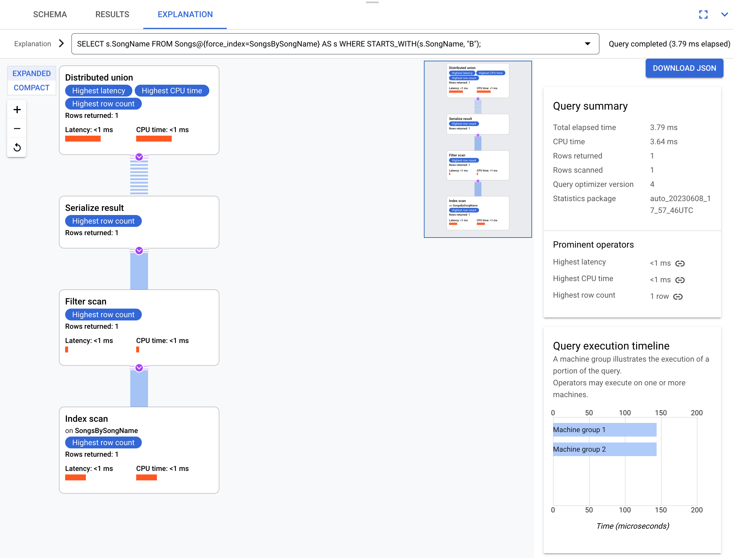
The execution plan doesn't require a back join because all the columns requested by the query are present in the index.

What's next

• Learn about Query execution operators

• Learn about the Spanner query optimizer

• Learn how to Manage the query optimizer