This document shows you how to find the right resource mappings from on-premises hardware to Google Cloud. In a scenario where your applications are running on bare-metal servers and you want to migrate them to Google Cloud, you might consider the following questions:
- How do physical cores (pCPUs) map to virtual CPUs (vCPUs) on Google Cloud? For example, how do you map 4 physical cores of bare-metal Xeon E5 to vCPUs in Google Cloud?
- How do you account for performance differences between different CPU platforms and processor generations? For example, is a 3.0 GHz Sandy Bridge 1.5 times faster than a 2.0 GHz Skylake?
- How do you right-size resources based on your workloads? For example, how can you optimize a memory-intensive, single-threaded application that's running on a multi-core server?
Sockets, CPUs, cores, and threads
The terms socket, CPU, core, and thread are often used interchangeably, which can cause confusion when you are migrating between different environments.
Simply put, a server can have one or more sockets. A socket (also called a CPU socket or CPU slot) is the connector on the motherboard that houses a CPU chip and provides physical connections between the CPU and the circuit board.
A CPU refers to the actual integrated circuit (IC). The fundamental operation of a CPU is to execute a sequence of stored instructions. At a high level, CPUs follow the fetch, decode, and execute steps, which are collectively known as the instruction cycle. In more complex CPUs, multiple instructions can be fetched, decoded, and executed simultaneously.
Each CPU chip can have one or more cores. A core essentially consists of an execution unit that receives instructions and performs actions based on those instructions. In a hyper-threaded system, a physical processor core allows its resources to be allocated as multiple logical processors. In other words, each physical processor core is presented as two virtual (or logical) cores to the operating system.
The following diagram shows a high-level view of a quad-core CPU with hyper-threading enabled.

In Google Cloud, each vCPU is implemented as a single hyper-thread on one of the available CPU platforms.
To find the total number of vCPUs (logical CPUs) in your system, you can use the following formula:
vCPUs = threads per physical core × physical cores per socket × number of sockets
The
lscpu
command gathers information that includes the number of sockets, CPUs, cores,
and threads. It also includes information about the CPU caches and cache
sharing, family, model, and
BogoMips.
Here's some typical output:
...
Architecture:           x86_64
CPU(s):                 1
On-line CPU(s) list:    0
Thread(s) per core:     1
Core(s) per socket:     1
Socket(s):              1
CPU MHz:                2200.000
BogoMIPS:               4400.00
...
When you map CPU resources between your existing environment and Google Cloud, make sure that you know how many physical or virtual cores your server has. For more information, see the Mapping resources section.
CPU clock rate
For a program to execute, it must be broken down into a set of instructions that the processor understands. Consider the following C program that adds two numbers and displays the result:
#include <stdio.h>
int main()
{
        int a = 11, b = 8;
        printf("%d \n", a+b);
}
On compilation, the program is converted into the following assembly code:
...
main:
.LFB0:
        .cfi_startproc
        pushq   %rbp
        .cfi_def_cfa_offset 16
        .cfi_offset 6, -16
        movq    %rsp, %rbp
        .cfi_def_cfa_register 6
        subq    $16, %rsp
        movl    $11, -8(%rbp)
        movl    $8, -4(%rbp)
        movl    -8(%rbp), %edx
        movl    -4(%rbp), %eax
        addl    %edx, %eax
        movl    %eax, %esi
        movl    $.LC0, %edi
        movl    $0, %eax
        call    printf
        movl    $0, %eax
        leave
        .cfi_def_cfa 7, 8
        ret
        .cfi_endproc
...
Each assembly instruction in the preceding output corresponds to a single
machine instruction. For example, the pushq instruction indicates that the
contents of the
RBP register
should be pushed onto the program stack. During each CPU cycle, a CPU can
perform a basic operation such as fetching an instruction, accessing the content
of a register, or writing data. To step through each stage of the cycle for
adding two numbers, see this
CPU simulator.
Note that each CPU instruction might require multiple clock cycles to execute. The average number of clock cycles required per instruction for a program is defined by cycles per instruction (CPI), like so:
cycles per instruction = number of CPU cycles used / number of instructions executed
Most modern CPUs can execute multiple instructions per clock cycle through instruction pipelining. The average number of instructions executed per cycle is defined by instructions per cycle (IPC), like so:
instructions per cycle = number of instructions executed / number of CPU cycles used
The CPU clock rate defines the number of clock cycles that the processor can execute per second. For example, a 3.0 GHz processor can execute 3 billion clock cycles per second. This means that every clock cycle takes ~0.3 nanoseconds to execute. During each clock cycle, a CPU can perform 1 or more instructions as defined by IPC.
Clock rates are commonly used to compare processor performances. Going by their literal definition (number of cycles executed per second), you might conclude that a higher number of clock cycles would mean that the CPU can do more work and hence perform better. This conclusion might be valid when comparing CPUs in the same processor generation. However, clock rates should not be used as a sole performance indicator when comparing CPUs across different processor families. A new-generation CPU might provide better performance even when it runs at a lower clock rate than prior-generation CPUs.
Clock rates and system performance
To better understand a processor's performance, it's important to look not just at the number of clock cycles but also at the amount of work a CPU can do per cycle. The total execution time of a CPU-bound program is not only dependent on the clock rate but also on other factors such as number of instructions to be executed, cycles per instruction or instructions per cycle, instruction set architecture, scheduling and dispatching algorithms, and programming language used. These factors can vary significantly from one processor generation to another.
To understand how CPU execution can vary across two different implementations, consider the example of a simple factorial program. One of the following programs is written in C and another in Python. Perf (a profiling tool for Linux) is used to capture some of the CPU and kernel metrics.
C program
#include <stdio.h>
int main()
{
    int n=7, i;
    unsigned int factorial = 1;
    for(i=1; i<=n; ++i){
            factorial *= i;
    }

    printf("Factorial of %d = %d", n, factorial);
}

Performance counter stats for './factorial':

...
0             context-switches       #    0.000 K/sec
0             cpu-migrations         #    0.000 K/sec
45            page-faults            #    0.065 M/sec
1,562,075     cycles                 #    1.28 GHz
1,764,632     instructions           #    1.13  insns per cycle
314,855       branches               #    257.907 M/sec
8,144         branch-misses          #    2.59% of all branches
...

0.001835982 seconds time elapsed
Python program
num = 7
factorial = 1
for i in range(1,num + 1):
  factorial = factorial*i
print("The factorial of",num,"is",factorial)

Performance counter stats for 'python3 factorial.py':

...
7              context-switches      #    0.249 K/sec
0              cpu-migrations        #    0.000 K/sec
908            page-faults           #    0.032 M/sec
144,404,306    cycles                #    2.816 GHz
158,878,795    instructions          #    1.10  insns per cycle
38,254,589     branches              #    746.125 M/sec
945,615        branch-misses         #    2.47% of all branches
...

0.029577164 seconds time elapsed
The highlighted output shows the total time taken to execute each program. The program written in C executed ~15 times faster than the program written in Python (1.8 milliseconds vs. 30 milliseconds). Here are some additional comparisons:
Context switches. When the system scheduler needs to run another program or when an interrupt triggers an on-going execution, the operating system saves the running program's CPU register contents and sets them up for the new program execution. No context switches occurred during the C program's execution, but 7 context switches occurred during the Python program's execution.
CPU migrations. The operating system tries to maintain workload balance among the available CPUs in multi-processor systems. This balancing is done periodically and every time a CPU run queue is empty. During the test, no CPU migration was observed.
Instructions. The C program resulted in 1.7 million instructions that were executed in 1.5 million CPU cycles (IPC = 1.13, CPI = 0.88), whereas the Python program resulted in 158 million instructions that were executed in 144 million cycles (IPC = 1.10, CPI = 0.91). Both programs filled up the pipeline, allowing the CPU to run more than 1 instruction per cycle. But compared to C, the number of instructions generated for Python is ~90 times greater.
Page faults. Each program has a slice of virtual memory that contains all of its instructions and data. Usually, it's not efficient to copy all of these instructions in the main memory at once. A page fault happens each time a program needs part of its virtual memory's content to be copied in the main memory. A page fault is signaled by the CPU through an interrupt.
Because the interpreter executable for Python is much bigger than for C, the additional overhead is evident both in terms of CPU cycles (1.5M for C, 144M for Python) and page faults (45 for C, 908 for Python).
Branches and branch-misses. For conditional instructions, the CPU tries to predict the execution path even before evaluating the branching condition. Such a step is useful to keep the instruction pipeline filled. This process is called speculative execution. The speculative execution was quite successful in the preceding executions: the branch predictor was wrong only 2.59% of the time for the program in C, and 2.47% of the time for the program in Python.
Factors other than CPU
So far, you've looked at various aspects of CPUs and their impact on
performance. However, it's rare for an application to have sustained on-CPU
execution 100% of the time. As a simple example, consider the following tar
command that creates an archive from a user's home directory in Linux:
$ time tar cf archive.tar /home/"$(whoami)"
The output looks like this:
real  0m35.798s
user  0m1.146s
sys   0m6.256s
These output values are defined as follows:
- real time
- Real time (
real) is the amount of time the execution takes from start to finish. This elapsed time includes time slices used by other processes and the time when the process is blocked, for example, when it's waiting for I/O operations to complete. - user time
- User time (
user) is the amount of CPU time spent executing user-space code in the process. - system time
- System time (
sys) is the amount of CPU time spent executing kernel-space code in the process.
In the preceding example, the user time is 1.0 second, while the system time is
6.3 seconds. The ~28 seconds difference between real time and user + sys
time points to the off-CPU time spent by the tar command.
A high off-CPU time for an execution indicates that the process is not CPU bound. Computation is said to be bound by something when that resource is the bottleneck for achieving the expected performance. When you plan a migration, it's important to have a holistic view of the application and to consider all the factors that can have a meaningful impact on performance.
Role of target workload in migration
In order to find a reasonable starting point for the migration, it's important to benchmark the underlying resources. You can do performance benchmarking in various ways:
Actual target workload: Deploy the application in the target environment and benchmark performance of the key performance indicators (KPIs). For example, KPIs for a web application can include the following:
- Application load time
- End-user latencies for end-to-end transactions
- Dropped connections
- Number of serving instances for low, average, and peak traffic
- Resource (CPU, RAM, disk, network) utilization of serving instances
However, deploying a full (or a subset of) target application can be complex and time consuming. For preliminary benchmarking, program-based benchmarks are generally preferred.
Program-based benchmarks: Program-based benchmarks focus on individual components of the application rather than the end-to-end application flow. These benchmarks run a mix of test profiles, where each profile is targeted toward one component of the application. For example, test profiles for a LAMP stack deployment can include Apache Bench, which is used to benchmark the web server performance, and Sysbench, which is used to benchmark MySQL. These tests are generally easier to set up than actual target workloads and are highly portable across different operating systems and environments.
Kernel or synthetic benchmarks: To test key computationally intensive aspects from real programs, you can use synthetic benchmarks such as matrix factorization or FFT. You typically run these tests during the early application design phase. They are best suited for benchmarking only certain aspects of a machine such as VM and drive stress, I/O syncs, and cache thrashing.
Understanding your application
Many applications are bound by CPU, memory, disk I/O, and network I/O, or a combination of these factors. For example, if an application is experiencing slowness due to contention on disks, providing more cores to the servers might not improve performance.
Note that maintaining observability for applications over large, complex environments can be nontrivial. There are specialized monitoring systems that can keep track of all distributed, system-wide resources. For example, on Google Cloud you can use Cloud Monitoring to get full visibility across your code, applications, and infrastructure. A Cloud Monitoring example is discussed later in this section, but first it's a good idea to understand monitoring of typical system resources on a standalone server.
Many utilities such as
top,
IOStat,
VMStat,
and
iPerf
can provide a high-level view of a system's resources. For example, running
top on a Linux system produces an output like this:
top - 13:20:42 up 22 days,  5:25,         18 users,        load average: 3.93 2.77,3.37
Tasks:  818 total,        1 running,      760 sleeping,    0 stopped,       0 zombie
Cpu(s): 88.2%us,          0.0%sy,         0.0%ni,          0.3%id,          0.0%wa, 0.0%hi, 0.0%si, 0.0%st
Mem:    49375504k total,  6675048k used,  42700456k free,  276332k buffers
Swap:   68157432k total,  0k used,        68157432k free,  5163564k cached
If the system has a high load and the wait-time percentage is high, you likely have an I/O-bound application. If either or both of user-percentage time or system-percentage time are very high, you likely have a CPU-bound application.
In the previous example, the load averages (for a 4 vCPU VM) in the last 5 minutes, 10 minutes, and 15 minutes are 3.93, 2.77, and 3.37 respectively. If you combine these averages with the high percentage of user time (88.2%), low idle time (0.3%), and no wait time (0.0%), you can conclude that the system is CPU bound.
Although these tools work well for standalone systems, they are typically not designed to monitor large, distributed environments. To monitor production systems, tools such as Cloud Monitoring, Nagios, Prometheus, and Sysdig can provide in-depth analysis of resource consumption against your applications.
Performance monitoring your application over a sufficient period of time lets you collect data across multiple metrics such as CPU utilization, memory usage, disk I/O, network I/O, roundtrip times, latencies, error rates, and throughput. For example, the following Cloud Monitoring graphs show CPU loads and utilization levels along with memory and disk usage for all servers running in a Google Cloud managed instance group. To learn more about this setup, see the Cloud Monitoring agent overview.

For analysis, the data-collection period should be long enough to show the peak and trough utilization of resources. You can then analyze the collected data to provide a starting point for capacity planning in the new target environment.
Map resources
This section walks through how to establish resource sizing on Google Cloud. First, you make an initial sizing assessment based on existing resource utilization levels. Then you run application-specific performance benchmarking tests.
Usage-based sizing
Follow these steps to map the existing core count of a server to vCPUs in Google Cloud.
Find the current core count. Refer to the
lscpucommand in the earlier sectionFind the CPU utilization of the server. CPU usage refers to the time that the CPU takes when it is in user mode (
%us) or kernel mode (%sy). Nice processes (%ni) also belong to user mode, whereas software interrupts (%si) and hardware interrupts (%hi) are handled in kernel mode. If the CPU isn't doing any of these, then either it's idle or waiting for I/O to complete. When a process is waiting for I/O to complete, it doesn't contribute to CPU cycles.To calculate the current CPU usage of a server, you run the following
topcommand:... Cpu(s): 88.2%us, 0.0%sy, 0.0%ni, 0.3%id, 0.0%wa, 0.0%hi, 0.0%si, 0.0%st ...CPU usage is defined as follows:
CPU Usage = %us + %sy + %ni + %hi + %siAlternatively, you can use any monitoring tool like Cloud Monitoring that can collect the required CPU inventory and utilization. For application deployments that are non-autoscaling (that is, run with one or more fixed number of servers), we recommend that you consider using peak utilization for CPU sizing. This approach safeguards application resources against disruptions when workloads are at peak utilization. For autoscaling deployments (based on CPU usage), average CPU utilization is a safe baseline to consider for sizing. In that case, you handle traffic spikes by scaling out the number of servers for the duration of the spike.
Allocate sufficient buffer to accommodate any spikes. When you are CPU sizing, include a sufficient buffer to accommodate any unscheduled processing that might cause unexpected spikes. For example, you can plan for CPU capacity such that there's additional headroom of 10–15% over expected peak usage, and the overall maximum CPU utilization doesn't exceed 70%.
Use the following formula to calculate the expected core count on GCP:
vCPUs on Google Cloud = 2 × CEILING[(core-count × utilization%) / (2 × threshold%)]
These values are defined as follows:
- core-count: The existing core count (as calculated in step 1).
- utilization%: The CPU utilization of the server (as calculated in step 2).
- threshold%: The maximum CPU usage allowed on the server after taking into account sufficient headroom (as calculated in step 3).
For a concrete example, consider a scenario where you have to map the core count
of a bare-metal
4-core Xeon E5640
server running on-premises to vCPUs in Google Cloud. Xeon E5640 specs are
available
publicly,
but you can also confirm this by running a command like lscpu on the system.
The numbers look like the following:
- existing core count on-premises = sockets (1) × cores (4) × threads per core (2) = 8.
- Suppose that the CPU utilization (utilization%) observed during peak traffic is 40%.
- There's a provision for an additional buffer of 30%; that is, maximum CPU utilization (threshold%) should not exceed 70%.
- vCPUs on Google Cloud = 2 × CEILING[(8 × 0.4)/(2 × 0.7)] = 6 vCPUs
(that is, 2 × CEILING[3.2/1.4] = 2 × CEILING[2.28] = 2 × 3 = 6)
You can do similar assessments for RAM, disk, network I/O, and other system resources.
Performance-based sizing
The previous section covered details of mapping pCPUs to vCPUs based on current and expected levels of CPU use. This section considers the application that's running on the server.
In this section, you run a standard, canonical set of tests (program-based benchmarks) in order to benchmark performance. Continuing with the example scenario, consider that you are running a MySQL server on the Xeon E5 machine. In this case, you can use Sysbench OLTP to benchmark the database performance.
A simple read-write test on MySQL using Sysbench produces the following output:
OLTP test statistics:
  queries performed:
    read:              520982
    write:             186058
    other:             74424
    total:             781464
  transactions:        37211 (620.12 per sec.)
  deadlocks:           2 (0.03 per sec.)
  read/write requests: 707040 (11782.80 per sec.)
  other operations:    74424 (1240.27 per sec.)

Test execution summary:
  total time:          60.0061s
  total number of events: 37211
  total time taken by event execution: 359.8158
  per-request statistics:
    min:            2.77ms
    avg:            9.67ms
    max:            50.81ms
    approx. 95 percentile: 14.63ms

Thread fairness:
  events (avg/stddev):         6201.8333/31.78
  execution time (avg/stddev): 59.9693/0.00
Running this benchmark lets you compare performance in terms of number of transactions per second, total reads/writes per second, and end-to-end execution time between your current environment and Google Cloud. We recommend that you run multiple iterations of these tests in order to rule out any outliers. To observe performance differences under varying load and traffic patterns, you can also repeat these tests with different parameters, such as concurrency levels, duration of tests, and number of simulated users or varying hatch rates.
The performance numbers between the current environment and Google Cloud will help further rationalize your initial capacity assessment. If the benchmarking tests on Google Cloud yield similar or better results than the existing environment, then you can further adjust the scale of resources based on the performance gains. On the other hand, if benchmarks on your existing environment are better than on Google Cloud, you should do the following:
- Revisit the initial capacity assessment.
- Monitor system resources.
- Find possible areas of contention (for example, bottlenecks identified on CPU and RAM).
- Resize resources accordingly.
After you're done, rerun your application-specific benchmark tests.
End-to-end performance benchmarking
So far, you've looked at a simplistic scenario that compared just the MySQL performance between on-premises and Google Cloud. In this section, you consider the following distributed 3-tier application.

As the diagram shows, you've likely run multiple benchmarks to reach a reasonable assessment of your current environment and Google Cloud. However, it can be challenging to establish which subset of benchmarks estimates your application performance most accurately. Furthermore, it can be a tedious task to manage the test process from dependency management to test installation, execution, and result aggregation across different cloud or non-cloud environments. For such scenarios, you can use PerfKitBenchmarker. PerfKit contains various sets of benchmarks to measure and compare different offerings across multiple clouds. It can also run certain benchmarks on-premises through static machines.
Suppose that for the 3-tier application in the preceding diagram, you want to run tests to benchmark cluster boot time, CPU, and network performance of VMs on Google Cloud. Using PerfKitBenchmarker, you can run multiple iterations of relevant test profiles, which produce the following results:
Cluster boot time: Provides a view of VM boot time. This is particularly important if the application is elastic and expects instances to be added or removed as part of autoscaling. The following graph shows that the boot times of an
n1-standard-4Compute Engine instance stay fairly consistent (up to the 99th percentile) at 40–45 seconds.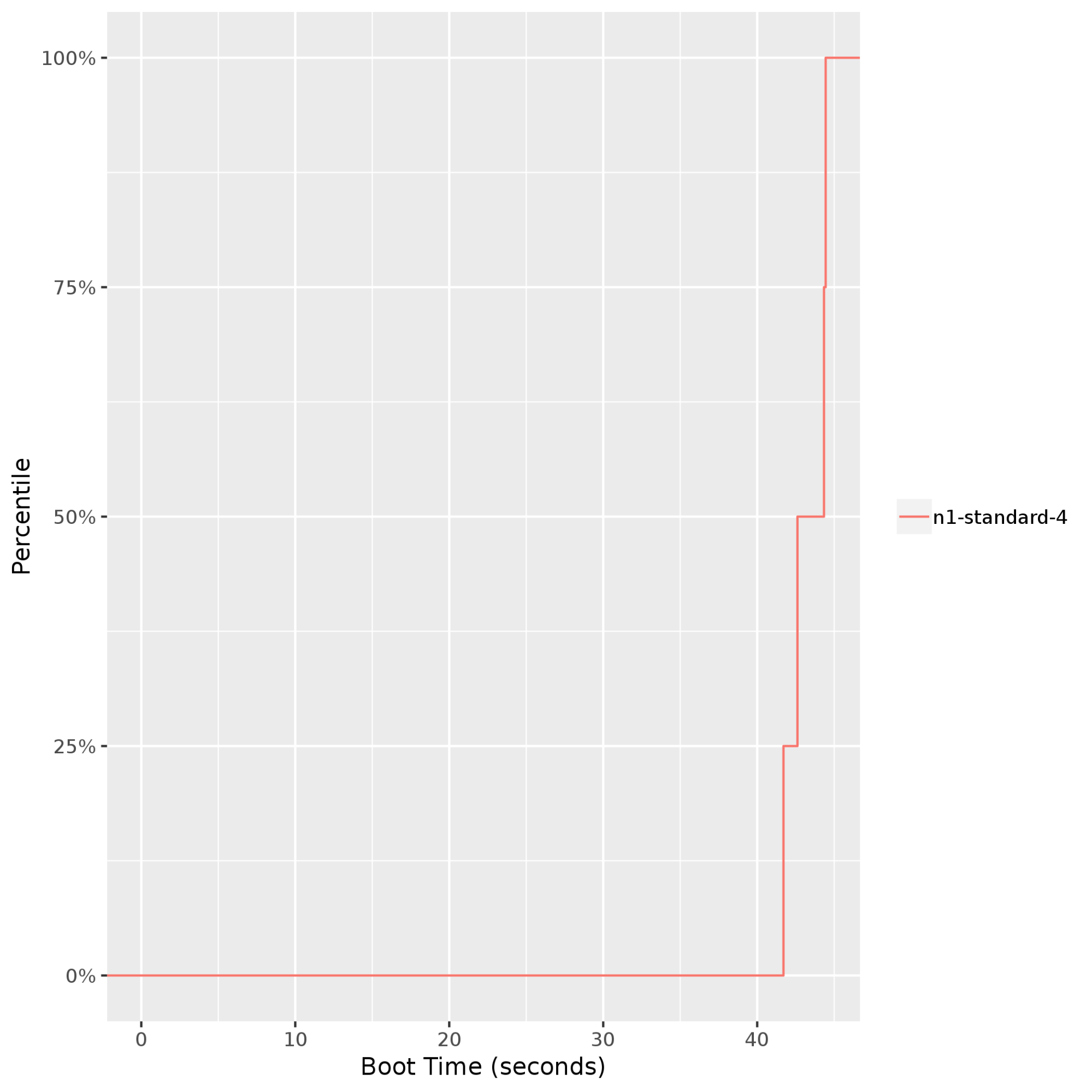
Stress-ng: Measures and compares compute-intensive performance by stressing a system's processor, memory subsystem, and compiler. In the following example,stress-ngruns multiple stress tests such asbsearch,malloc,matrix,mergesort, andzlibon ann1-standard-4Compute Engine instance.Stress-ngmeasures stress-test throughput using bogus operations (bogo ops) per second. If you normalize bogo ops across different stress test results, you get the following output, which shows the geometric mean of operations executed per second. In this example, bogo ops range from ~8,000 per second at the 50th percentile to ~10,000 per second at the 95th percentile. Note that bogo ops are generally used to benchmark only standalone CPU performance. These operations might not be representative of your application.
Netperf: Measures latency with request and response tests. Request and response tests run at the application layer of the network stack. This method of latency testing involves all of the layers of the stack and is preferred over ping tests to measure VM-to-VM latency. The following graph shows the TCP request and response (TCP_RR) latencies between a client and server that are running in the same Google Cloud zone. TCP_RR values range from ~70 microseconds at the 50th percentile to ~130 microseconds at the 90th percentile.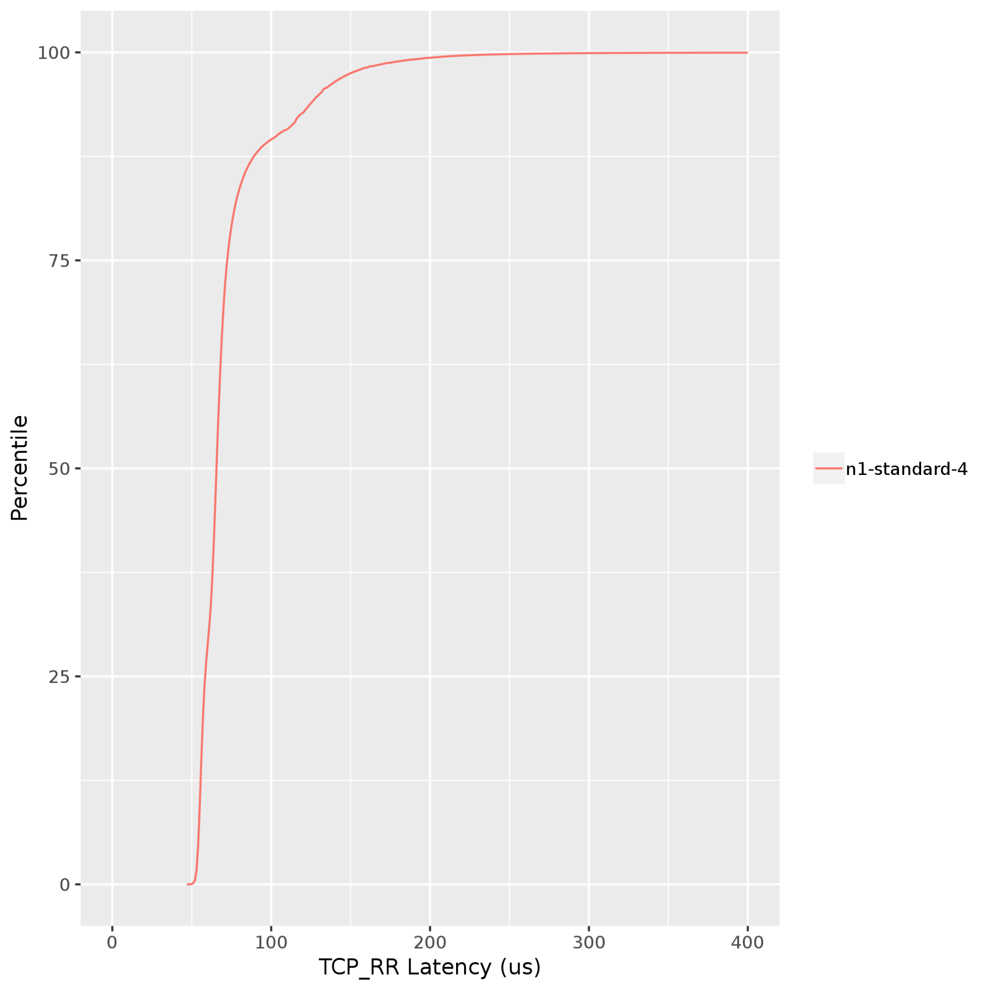
Given the nature of the target workload, you can run other test profiles by using PerfKit. For details, see supported benchmarks in PerfKit.
Best practices on Google Cloud
Before you set up and execute a migration plan on Google Cloud, we recommend that you follow the migration best practices. These practices are only a starting point. You might need to consider many other aspects of your application—such as decoupling dependencies, introducing fault tolerance, and ensuring scale-up and scale-down based on component workload—and how each of those aspects map to Google Cloud.
Know Google Cloud limits and quotas. Before formally starting with capacity assessment, understand some important considerations for resource planning on Google Cloud—for example:
- Per-instance network quotas
- Disk performance on Google Cloud
- Available CPU platforms on Google Cloud
List the infrastructure as a service (IaaS) and platform as a service (PaaS) components that would be required during the migration and clearly understand any quotas and limits and any fine-tuning adjustments available with each of the services.
Monitor resources continuously. Continuous resource monitoring can help you identify patterns and trends in system and application performance. Monitoring not only helps establish baseline performance but also demonstrates the need for hardware upgrades and downgrades over time. Google Cloud provides various options to deploy end-to-end monitoring solutions:
Right-size your VMs. Identify when a VM is under-provisioned or over-provisioned. Setting up basic monitoring as discussed earlier should easily provide these insights. Google Cloud also provides right-sizing recommendations based on an instance's historical usage. Furthermore, based on the nature of the workload, if predefined machine types don't meet your needs, you can create an instance with custom virtualized hardware settings.
Use the right tools. For large-scale environments, deploy automated tools to minimize manual effort—for example:
- StratoZone and CloudPhysics for application discovery and existing inventory data collection.
- Migrate to Virtual Machines to migrate VMs to Google Cloud and for built-in testing to validate in-cloud performance, SLAs, and cost.
- Database Migration Service to migrate data and databases to Google Cloud.
- Cloud Deployment Manager to provision cloud infrastructure resources as code (IaC).
Takeaways
Migrating resources from one environment to another requires careful planning. It's important to not look at hardware resources in isolation but to take an end-to-end view of your application. For example, instead of solely focusing on whether a 3.0 GHz Sandy Bridge processor is going to be twice as fast as a 1.5 GHz Skylake processor, focus instead on how your application's key performance indicators change from one computing platform to another.
When you assess resource mapping requirements across different environments, consider the following:
- System resources that your application is constrained by (for example, CPU, memory, disk, or network).
- Impact of the underlying infrastructure (for example, processor generation, clock speed, HDD or SSD) on the performance of your application.
- Impact of software and architectural design choices (for example, single or multithreaded workloads, fixed or autoscaling deployments) on the performance of the application.
- Current and expected utilization levels of compute, storage, and network resources.
- Most appropriate performance tests that are representative of your application.
Collecting data against these metrics through continuous monitoring helps you determine an initial capacity plan. You can follow up by doing appropriate performance benchmarking to fine-tune your initial sizing estimates.
What's next
- Learn more about best practices for migrating VMs to Google Cloud.
- Read about Google Cloud's migration center.
- Learn more about the Cloud Foundation Toolkit.
- Learn more about how to get started with Google Cloud migration.
- Learn more about how Google Cloud compares with other cloud platforms.
- Explore reference architectures, diagrams, and best practices about Google Cloud. Take a look at our Cloud Architecture Center.