Data science with R on Google Cloud: Exploratory data analysis tutorial

Last reviewed 2024-04-16 UTC

---

This tutorial shows you how to get started with data science at scale with R on Google Cloud. This is intended for those who have some experience with R and with Jupyter notebooks, and who are comfortable with SQL.

This tutorial focuses on performing exploratory data analysis using Vertex AI Workbench user-managed notebooks and BigQuery. You can find the code for this tutorial in a Jupyter notebook that's on GitHub.

Overview

R is one of the most widely used programming languages for statistical modeling. It has a large and active community of data scientists and machine learning (ML) professionals. With over 15,000 packages in the open-source repository of the Comprehensive R Archive Network (CRAN), R has tools for all statistical data analysis applications, ML, and visualization. R has experienced steady growth in the last two decades due to its expressiveness of its syntax, and because of how comprehensive its data and ML libraries are.

As a data scientist, you might want to know how you can make use of your skill set by using R, and how you can also harness the advantages of the scalable, fully managed cloud services for ML.

Architecture

In this tutorial, you use user-managed notebooks as the data science environment to perform exploratory data analysis (EDA). You use R on data that you extract as part of this tutorial from BigQuery, Google's serverless, highly scalable, and cost-effective cloud data warehouse. After you analyze and process the data, the transformed data is stored in Cloud Storage for further ML tasks. This flow is shown in the following diagram:

Data for the tutorial

The dataset used in this tutorial is the BigQuery natality dataset. This public dataset includes information about more than 137 million births registered in the United States from 1969 to 2008.

This tutorial focuses on EDA and on visualization using R and BigQuery. The tutorial sets you up for a machine-learning goal of predicting a baby's weight given a number of factors about the pregnancy and about the baby's mother, although that task is not covered in this tutorial.

User-managed notebooks

Vertex AI Workbench user-managed notebooks is a service that offers an integrated JupyterLab environment, with the following features:

• One-click deployment. You can use a single click to start a JupyterLab instance that's preconfigured with the latest machine-learning and data-science frameworks.
• Scale on demand. You can start with a small machine configuration (for example, 4 vCPUs and 15 GB of RAM, as in this tutorial), and when your data gets too big for one machine, you can scale up by adding CPUs, RAM, and GPUs.
• Google Cloud integration. Vertex AI Workbench user-managed notebooks instances are integrated with Google Cloud services like BigQuery. This integration makes it easy to go from data ingestion to preprocessing and exploration.
• Pay-per-use pricing. There are no minimum fees or up-front commitments. See pricing for Vertex AI Workbench user-managed notebooks. You also pay for the Google Cloud resources that you use with the user-managed notebooks instance.

User-managed notebooks runs on Deep Learning VM Images. These images are optimized to support ML frameworks like PyTorch and TensorFlow. This tutorial supports creating a user-managed notebooks instance that has R 3.6.

Working with BigQuery using R

BigQuery doesn't require infrastructure management, so you can focus on uncovering meaningful insights. BigQuery lets you use familiar SQL to work with your data, so you don't need a database administrator. You can use BigQuery to analyze large amounts of data at scale, and to prepare datasets for ML using BigQuery's rich SQL analytical capabilities.

To query BigQuery data using R, you can use bigrquery, an open-source R library. The bigrquery package provides the following levels of abstraction on top of BigQuery:

• The low-level API provides thin wrappers over the underlying BigQuery REST API.

• The DBI interface wraps the low-level API and makes working with BigQuery similar to working with any other database system. This is the most convenient layer if you want to run SQL queries in BigQuery or upload less than 100 MB.

• The dbplyr interface lets you treat BigQuery tables like in-memory data frames. This is the most convenient layer if you don't want to write SQL, but instead want dbplyr to write it for you.

This tutorial uses the low-level API from bigrquery, without requiring DBI or dbplyr.

Objectives

• Create a user-managed notebooks instance that has R support.
• Query and analyze data from BigQuery using the bigrquery R library.
• Prepare and store data for ML in Cloud Storage.

Costs

In this document, you use the following billable components of Google Cloud:

• BigQuery
• Vertex AI Workbench user-managed notebooks instance. You are also charged for resources used within notebooks, including compute resources, BigQuery, and API requests.
• Cloud Storage

To generate a cost estimate based on your projected usage, use the pricing calculator. New Google Cloud users might be eligible for a free trial.

Before you begin

1. Sign in to your Google Cloud account. If you're new to Google Cloud, create an account to evaluate how our products perform in real-world scenarios. New customers also get $300 in free credits to run, test, and deploy workloads.

2. In the Google Cloud console, on the project selector page, select or create a Google Cloud project.

   Note: If you don't plan to keep the resources that you create in this procedure, create a project instead of selecting an existing project. After you finish these steps, you can delete the project, removing all resources associated with the project.

   Go to project selector

3. Make sure that billing is enabled for your Google Cloud project.

4. Enable the Compute Engine API.

   Enable the API

5. In the Google Cloud console, on the project selector page, select or create a Google Cloud project.

   Note: If you don't plan to keep the resources that you create in this procedure, create a project instead of selecting an existing project. After you finish these steps, you can delete the project, removing all resources associated with the project.

   Go to project selector

6. Make sure that billing is enabled for your Google Cloud project.

7. Enable the Compute Engine API.

   Enable the API

Creating a user-managed notebooks instance with R

The first step is to create a user-managed notebooks instance that you can use for this tutorial.

1. In the Google Cloud console, go to the Notebooks page.

   Go to Notebooks

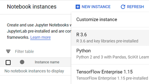
2. On the User-managed notebooks tab, click  New notebook.

3. Select R 3.6.

   

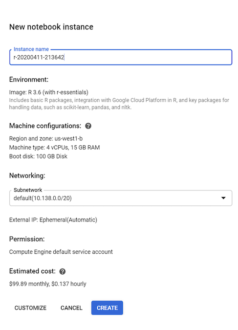
4. For this tutorial, leave all the default values and click Create:

   

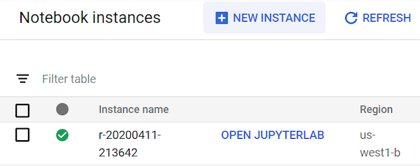
   The user-managed notebooks instance can take up to 90 seconds to start. When it's ready, you see it listed in the Notebook instances pane with an Open JupyterLab link next to the instance name:

   

Opening JupyterLab

To go through the tutorial in the notebook, you need to open the JupyterLab environment, clone the ml-on-gcp GitHub repository, and then open the notebook.

1. In the instances list, click Open Jupyterlab. This opens the JupyterLab environment in your browser.

   

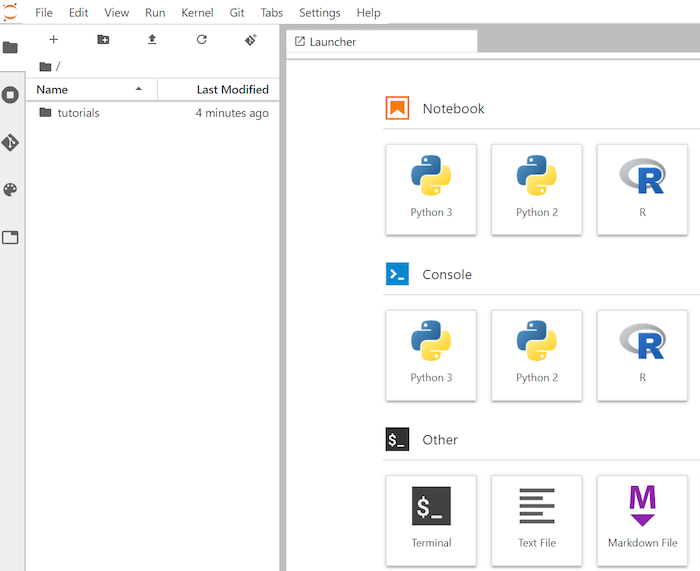
2. To launch a terminal tab, click Terminal in the Launcher.

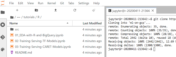
3. In the terminal, clone the ml-on-gcp GitHub repository:

   git clone https://github.com/GoogleCloudPlatform/ml-on-gcp.git
   

   When the command finishes, you see the ml-on-gcp folder in the file browser.

4. In the file browser, open ml-on-gcp, then tutorials, and then R.

   The result of cloning looks like the following:

   

Opening the notebook and setting up R

The R libraries that you need for this tutorial, including bigrquery, are installed in R notebooks by default. As part of this procedure, you import them to make them available to the notebook.

1. In the file browser, open the 01-EDA-with-R-and-BigQuery.ipynb notebook.

   This notebook covers the exploratory data analysis tutorial with R and BigQuery. From this point in the tutorial, you work in the notebook, and you run the code you see within the Jupyter notebook itself.

2. Import the R libraries that you need for this tutorial:

   library(bigrquery) # used for querying BigQuery
   library(ggplot2) # used for visualization
   library(dplyr) # used for data wrangling
   

3. Authenticate bigrquery using out-of-band authentication:

   bq_auth(use_oob = True)
   

4. Set a variable to the name of the project you use for this tutorial:

   # Set the project ID
   PROJECT_ID <- "gcp-data-science-demo"
   

5. Set a variable to the name of the Cloud Storage bucket:

   BUCKET_NAME <- "bucket-name"
   

   Replace bucket-name with a name that's globally unique.

   You use the bucket later to store the output data.

Querying data from BigQuery

In this section of the tutorial, you read the results of executing a BigQuery SQL statement into R and take a preliminary look at the data.

1. Create a BigQuery SQL statement that extracts some possible predictors and the target prediction variable for a sample of births since 2000:

   sql_query <- "
       SELECT
         ROUND(weight_pounds, 2) AS weight_pounds,
         is_male,
         mother_age,
         plurality,
         gestation_weeks,
         cigarette_use,
         alcohol_use,
         CAST(ABS(FARM_FINGERPRINT(CONCAT(
           CAST(YEAR AS STRING), CAST(month AS STRING),
           CAST(weight_pounds AS STRING)))
           ) AS STRING) AS key
       FROM
           publicdata.samples.natality
       WHERE
         year > 2000
         AND weight_pounds > 0
         AND mother_age > 0
         AND plurality > 0
         AND gestation_weeks > 0
         AND month > 0
       LIMIT %s
   "
   

   The key column is a generated row identifier based on the concatenated values of the year, month, and weight_pounds columns.

2. Run the query and retrieve the data as an in-memory data frame object:

   sample_size <- 10000
   sql_query <- sprintf(sql_query, sample_size)
   
   natality_data <- bq_table_download(
       bq_project_query(
           PROJECT_ID,
           query=sql_query
       )
   )
   

3. View the retrieved results:

   head(natality_data)
   

   The output is similar to the following:

   

4. View the number of rows and data types of each column:

   str(natality_data)
   

   The output is similar to the following:

   Classes ‘tbl_df’, ‘tbl’ and 'data.frame':   10000 obs. of  8 variables:
    $ weight_pounds  : num  7.75 7.4 6.88 9.38 6.98 7.87 6.69 8.05 5.69 9.22 ...
    $ is_male        : logi  FALSE TRUE TRUE TRUE FALSE TRUE ...
    $ mother_age     : int  47 44 42 43 42 43 42 43 45 44 ...
    $ plurality      : int  1 1 1 1 1 1 1 1 1 1 ...
    $ gestation_weeks: int  41 39 38 39 38 40 35 40 38 39 ...
    $ cigarette_use  : logi  NA NA NA NA NA NA ...
    $ alcohol_use    : logi  FALSE FALSE FALSE FALSE FALSE FALSE ...
    $ key            : chr  "3579741977144949713" "8004866792019451772" "7407363968024554640" "3354974946785669169" ...
   

5. View a summary of the retrieved data:

   summary(natality_data)
   

   The output is similar to the following:

    weight_pounds     is_male          mother_age     plurality
    Min.   : 0.620   Mode :logical   Min.   :13.0   Min.   :1.000
    1st Qu.: 6.620   FALSE:4825      1st Qu.:22.0   1st Qu.:1.000
    Median : 7.370   TRUE :5175      Median :27.0   Median :1.000
    Mean   : 7.274                   Mean   :27.3   Mean   :1.038
    3rd Qu.: 8.110                   3rd Qu.:32.0   3rd Qu.:1.000
    Max.   :11.440                   Max.   :51.0   Max.   :4.000
    gestation_weeks cigarette_use   alcohol_use         key
    Min.   :18.00   Mode :logical   Mode :logical   Length:10000
    1st Qu.:38.00   FALSE:580       FALSE:8284      Class :character
    Median :39.00   TRUE :83        TRUE :144       Mode  :character
    Mean   :38.68   NA's :9337      NA's :1572
    3rd Qu.:40.00
    Max.   :47.00
   

Visualizing data using ggplot2

In this section, you use the ggplot2 library in R to study some of the variables from the natality data set.

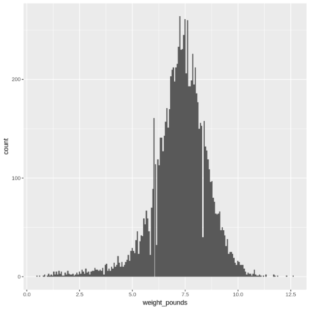
1. Display the distribution of the weight_pounds values using a histogram:

   ggplot(
       data = natality_data,
       aes(x = weight_pounds)
   ) + geom_histogram(bins = 200)
   

   The resulting plot is similar to the following:

   

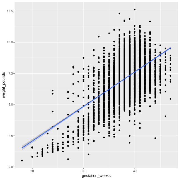
2. Display the relationship between gestation_weeks and weight_pounds using a scatter plot:

   ggplot(
       data = natality_data,
       aes(x = gestation_weeks, y = weight_pounds)
   ) + geom_point() + geom_smooth(method = "lm")
   

   The resulting plot is similar to the following:

   

Processing the data in BigQuery from R

When you're working with large datasets, we recommend that you perform as much analysis as possible (aggregation, filtering, joining, computing columns, and so on) in BigQuery and then retrieve the results. Performing these tasks in R is less efficient. Using BigQuery for analysis takes advantage of the scalability and performance of BigQuery, and makes sure that the returned results can fit into memory in R.

1. Create a function that finds the number of records and the average weight for each value of the chosen column:

   get_distinct_values <- function(column_name) {
       query <- paste0(
           'SELECT ', column_name, ',
               COUNT(1) AS num_babies,
               AVG(weight_pounds) AS avg_wt
           FROM publicdata.samples.natality
           WHERE year > 2000
           GROUP BY ', column_name)
   
       bq_table_download(
           bq_project_query(
               PROJECT_ID,
               query = query
           )
       )
   }
   

2. Invoke this function using the mother_age column and then look at the number of babies and average weight by mother age:

   df <- get_distinct_values('mother_age')
   ggplot(data = df, aes(x = mother_age, y = num_babies)) + geom_line()
   ggplot(data = df, aes(x = mother_age, y = avg_wt)) + geom_line()
   

   The output of the first ggplot command is as follows, showing the number of babies born by mother's age.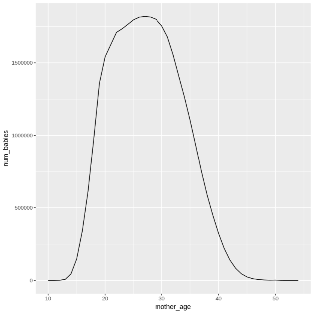

   

   The output of the second ggplot command is as follows, showing the the average weight of babies by mother's age.

   

To see more visualization examples, refer to the notebook.

Saving data as CSV files

The next task is to save extracted data from BigQuery as CSV files in Cloud Storage so you can use it for further ML tasks.

1. Load training and evaluation data from BigQuery into R:

   # Prepare training and evaluation data from BigQuery
   sample_size <- 10000
   sql_query <- sprintf(sql_query, sample_size)
   
   train_query <- paste('SELECT * FROM (', sql_query,
     ') WHERE MOD(CAST(key AS INT64), 100) <= 75')
   eval_query <- paste('SELECT * FROM (', sql_query,
     ') WHERE MOD(CAST(key AS INT64), 100) > 75')
   
   # Load training data to data frame
   train_data <- bq_table_download(
       bq_project_query(
           PROJECT_ID,
           query = train_query
       )
   )
   
   # Load evaluation data to data frame
   eval_data <- bq_table_download(
       bq_project_query(
           PROJECT_ID,
           query = eval_query
       )
   )
   

2. Write the data to a local CSV file:

   # Write data frames to local CSV files, without headers or row names
   dir.create(file.path('data'), showWarnings = FALSE)
   write.table(train_data, "data/train_data.csv",
      row.names = FALSE, col.names = FALSE, sep = ",")
   write.table(eval_data, "data/eval_data.csv",
      row.names = FALSE, col.names = FALSE, sep = ",")
   

3. Upload the CSV files to Cloud Storage by wrapping gsutil commands that are passed to the system:

   # Upload CSV data to Cloud Storage by passing gsutil commands to system
   gcs_url <- paste0("gs://", BUCKET_NAME, "/")
   command <- paste("gsutil mb", gcs_url)
   system(command)
   gcs_data_dir <- paste0("gs://", BUCKET_NAME, "/data")
   command <- paste("gsutil cp data/*_data.csv", gcs_data_dir)
   system(command)
   command <- paste("gsutil ls -l", gcs_data_dir)
   system(command, intern = TRUE)
   

   Another option for this step is to use the googleCloudStorageR library to do this by using the Cloud Storage JSON API.

Clean up

To avoid incurring charges to your Google Cloud account for the resources used in this tutorial, you should remove them.

Delete the project

The easiest way to eliminate billing is to delete the project you created for the tutorial.

Caution: Deleting a project has the following effects:

• Everything in the project is deleted. If you used an existing project for the tasks in this document, when you delete it, you also delete any other work you've done in the project.
• Custom project IDs are lost. When you created this project, you might have created a custom project ID that you want to use in the future. To preserve the URLs that use the project ID, such as an appspot.com URL, delete selected resources inside the project instead of deleting the whole project.

If you plan to explore multiple architectures, tutorials, or quickstarts, reusing projects can help you avoid exceeding project quota limits.

1. In the Google Cloud console, go to the Manage resources page.

   Go to Manage resources

2. In the project list, select the project that you want to delete, and then click Delete.
3. In the dialog, type the project ID, and then click Shut down to delete the project.

What's next

• Learn more about how you can use BigQuery data in your R notebooks in the bigrquery documentation.
• Learn about best practices for ML engineering in Rules of ML.
• Explore reference architectures, diagrams, and best practices about Google Cloud. Take a look at our Cloud Architecture Center.