Database replication using change data capture

Last reviewed 2020-10-20 UTC

This document describes several approaches to using change data capture (CDC) to integrate various data sources with BigQuery. This document provides an analysis of tradeoffs between data consistency, ease of use, and costs for each of the approaches. It will help you understand existing solutions, learn about different approaches to consume data that's replicated by CDC, and be able to create a cost-benefit analysis of the approaches.

This document is intended to help data architects, data engineers, and business analysts to develop an optimal approach for accessing replicated data in BigQuery. It assumes that you're familiar with BigQuery, SQL, and command-line tools.

Overview of CDC data replication

Databases like MySQL, Oracle, and SAP are the most often discussed CDC data sources. However, any system can be considered a data source if it captures and provides changes to data elements that are identified by primary keys. If a system doesn't provide a built-in CDC process, such as a transaction log, you can deploy an incremental batch reader to get changes.

This document discusses CDC processes that meet the following criteria:

1. Data replication captures changes for each table separately.
2. Every table has a primary key or a composite primary key.
3. Every emitted CDC event is assigned a monotonically increasing change ID, usually a numeric value like a transaction ID or a timestamp.
4. Every CDC event contains the complete state of the row that changed.

The following diagram shows a generic architecture using CDC for replicating data sources to BigQuery:

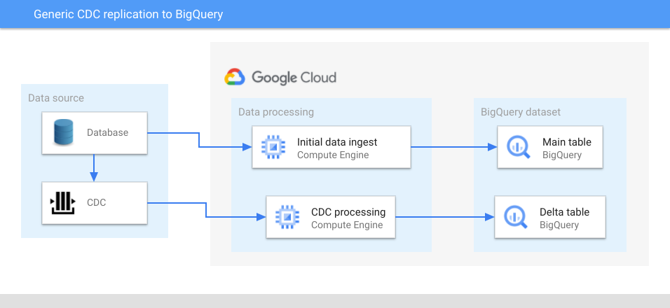
In the preceding diagram, a main table and a delta table are created in BigQuery for each source data table. The main table contains all of the source table's columns, plus one column for the latest change ID value. You can consider the latest change ID value as the version ID of the entity that's identified by the primary key of the record, and use it to find the latest version.

The delta table contains all of the source table's columns, plus an operation type column—one of update, insert, or delete—and the change ID value.

Following is the overall process to replicate data into BigQuery using CDC:

1. An initial data dump of a source table is extracted.
2. Extracted data is optionally transformed and then loaded into its corresponding main table. If the table doesn't have a column that can be used as a change ID, such as a last-updated timestamp, then the change ID is set to the lowest possible value for that column's data type. This lets subsequent processing identify the main table records that were updated after the initial data dump.
3. Rows that change after the initial data dump are captured by the CDC capture process.
4. If needed, additional data transformation is performed by the CDC processing layer. For example, the CDC processing layer might reformat the timestamp for use by BigQuery, split columns vertically, or remove columns.
5. The data is inserted into the corresponding delta table in BigQuery, using micro-batch loads or streaming inserts.

If additional transformations are performed before the data is inserted into BigQuery, the number and type of columns can differ from the source table. However, the same set of columns exist in the main and the delta tables.

Delta tables contain all change events for a particular table since the initial load. Having all change events available can be valuable for identifying trends, the state of the entities that a table represents at a particular moment, or change frequency.

To get the current state of an entity that's represented by a particular primary key, you can query the main table and the delta table for the record that has the most recent change ID. This query can be expensive because you might need to perform a join between the main and delta tables and complete a full table scan of one or both tables to find the most recent entry for a particular primary key. You can avoid performing a full table scan by clustering or partitioning the tables based on the primary key, but that isn't always possible.

This document compares the following generic approaches that can help you get the current state of an entity when you can't partition or cluster the tables:

• Immediate consistency approach: queries reflect the current state of replicated data. Immediate consistency requires a query that joins the main table and the delta table, and selects the most recent row for each primary key.
• Cost-optimized approach: faster and less expensive queries are executed at the expense of some delay in data availability. You can periodically merge the data into the main table.
• Hybrid approach: you use the immediate consistency approach or the cost optimized approach, depending on your requirements and budget.

The document discusses further ways to improve performance in addition to these approaches.

Before you begin

This document demonstrates using the bq command-line tool and SQL statements to view and query BigQuery data. Example table layouts and queries are shown later in this document. If you want to experiment with sample data, complete the following setup:

1. Select a project or create a project and enable billing for the project.
   • If you create a project, BigQuery is automatically enabled.
   • If you select an existing project, enable the BigQuery API.
2. In the Google Cloud console, open Cloud Shell.

3. To update your BigQuery configuration file, open the ~/.bigqueryrc file in a text editor and add or update the following lines anywhere in the file:

   [query]
   --use_legacy_sql=false
   
   [mk]
   --use_legacy_sql=false
   

4. Clone the GitHub repository that contains the scripts to set up the BigQuery environment:

   git clone https://github.com/GoogleCloudPlatform/bq-mirroring-cdc.git
   

5. Create the dataset, main, and delta tables:

   cd bq-mirroring-cdc/tutorial
   chmod +x *.sh
   ./create-tables.sh
   

To avoid potential charges when you're finished experimenting, shut down the project or delete the dataset.

Set up BigQuery data

To demonstrate different solutions for CDC data replication to BigQuery, you use a pair of main and delta tables that are populated with sample data like the following simple example tables.

To work with a more sophisticated setup than what's described in this document, you can use the CDC BigQuery integration demo. The demo automates the process of populating tables and it includes scripts to monitor the replication process. If you want to run the demo, follow the instructions in the README file that's in the root of the GitHub repository that you cloned in the Before you begin section of this document.

The example data uses a simple data model: a web session that contains a required system-generated session ID and an optional user name. When the session starts, the user name is null. After the user signs in, the user name is populated.

To load data into the main table from the BigQuery environment scripts, you can run a command like the following:

bq load cdc_tutorial.session_main init.csv

To get the main table contents, you can run a query like the following:

bq query "select * from cdc_tutorial.session_main limit 1000"

The output looks like the following:

+-----+----------+-----------+
| id  | username | change_id |
+-----+----------+-----------+
| 100 | NULL     |         1 |
| 101 | Sam      |         2 |
| 102 | Jamie    |         3 |
+-----+----------+-----------+

Next, you load the first batch of CDC changes into the delta table. To load the first batch of CDC changes to the delta table from the BigQuery environment scripts, you can run a command like the following:

bq load cdc_tutorial.session_delta first-batch.csv

To get the delta table contents, you can run a query like the following:

bq query "select * from cdc_tutorial.session_delta limit 1000"

The output looks like the following:

+-----+----------+-----------+-------------+
| id  | username | change_id | change_type |
+-----+----------+-----------+-------------+
| 100 | Cory     |         4 | U           |
| 101 | Sam      |         5 | D           |
| 103 | NULL     |         6 | I           |
| 104 | Jamie    |         7 | I           |
+-----+----------+-----------+-------------+

In the preceding output, the change_id value is the unique ID of a table row change. Values in the change_type column represent the following:

• U: update operations
• D: delete operations
• I: insert operations

The main table contains information about sessions 100, 101, and 102. The delta table has the following changes:

• Session 100 is updated with the username "Cory".
• Session 101 is deleted.
• New sessions 103 and 104 are created.

The current state of the sessions in the source system is as follows:

+-----+----------+
| id  | username |
+-----+----------+
| 100 | Cory     |
| 102 | Jamie    |
| 103 | NULL     |
| 104 | Jamie    |
+-----+----------+

Although the current state is displayed as a table, this table does not exist in materialized form. This table is the combination of the main and the delta table.

Query the data

There are multiple approaches you can use to determine the overall state of the sessions. The advantages and disadvantages of each approach are described in the following sections.

Immediate consistency approach

If immediate data consistency is your primary objective and the source data changes frequently, you can use a single query that joins the main and delta tables and selects the most recent row (the row with the most recent timestamp or the highest number value).

To create a BigQuery view that joins the main and delta tables and finds the most recent row, you can run a bq tool command like the following:

bq mk --view \
"SELECT * EXCEPT(change_type, row_num)
FROM (
  SELECT *, ROW_NUMBER() OVER (PARTITION BY id ORDER BY change_id DESC) AS row_num
  FROM (
    SELECT * EXCEPT(change_type), change_type
    FROM \`$(gcloud config get-value project).cdc_tutorial.session_delta\` UNION ALL
    SELECT *, 'I'
    FROM \`$(gcloud config get-value project).cdc_tutorial.session_main\`))
WHERE
  row_num = 1
  AND change_type <> 'D'" \
 cdc_tutorial.session_latest_v

The SQL statement in the preceding BigQuery view does the following:

• The innermost UNION ALL produces the rows from both the main and the delta tables:
  • SELECT * EXCEPT(change_type), change_type FROM session_delta forces the change_type column to be the last column in the list.
  • SELECT *, 'I' FROM session_main selects the row from the main table as if it were an insert row.
  • Using the * operator keeps the example simple. If there were additional columns or a different column order, replace the shortcut with explicit column lists.
• SELECT *, ROW_NUMBER() OVER (PARTITION BY id ORDER BY change_id DESC) AS row_num uses a window function in BigQuery to assign sequential row numbers starting with 1 to each of the groups of rows that have the same value of id, defined by PARTITION BY. The rows are ordered by change_id in descending order within that group. Because change_id is guaranteed to increase, the latest change has a row_num column that has a value of 1.
• WHERE row_num = 1 AND change_type <> 'D' selects only the latest row from each group. This is a common deduplication technique in BigQuery. This clause also removes the row from the result if its change type is delete.
• The topmost SELECT * EXCEPT(change_type, row_num) removes the extra columns that were introduced for processing and which aren't relevant otherwise.

The preceding example doesn't use the insert and update change types in the view because referencing the highest change_id value selects the original insert or the latest update. In this case, each row contains the complete data for all columns.

After you create the view, you can run queries against it. To get the most recent changes, you can run a query like the following:

bq query 'select * from cdc_tutorial.session_latest_v order by id limit 10'

The output looks like the following:

+-----+----------+-----------+
| id  | username | change_id |
+-----+----------+-----------+
| 100 | Cory     |         4 |
| 102 | Jamie    |         3 |
| 103 | NULL     |         6 |
| 104 | Jamie    |         7 |
+-----+----------+-----------+

When you query the view, the data in the delta table is immediately visible if you updated the data in the delta table using a data manipulation language (DML) statement, or almost immediately if you streamed data in.

Cost-optimized approach

The immediate consistency approach is simple, but it can be inefficient because it requires BigQuery to read all of the historical records, sort by primary key, and process the other operations in the query to implement the view. If you frequently query the session state, the immediate consistency approach could decrease performance and increase the costs of storing and processing data in BigQuery.

To minimize costs, you can merge delta table changes into the main table and periodically purge merged rows from the delta table. There is additional cost for merging and purging, but if you frequently query the main table, the cost is negligible compared to the cost of continuously finding the latest record for a key in the delta table.

To merge data from the delta table into the main table, you can run a MERGE statement like the following:

bq query \
'MERGE `cdc_tutorial.session_main` m
USING
  (
  SELECT * EXCEPT(row_num)
  FROM (
    SELECT *, ROW_NUMBER() OVER(PARTITION BY delta.id ORDER BY delta.change_id DESC) AS row_num
    FROM `cdc_tutorial.session_delta` delta )
  WHERE row_num = 1) d
ON  m.id = d.id
  WHEN NOT MATCHED
AND change_type IN ("I", "U") THEN
INSERT (id, username, change_id)
VALUES (d.id, d.username, d.change_id)
  WHEN MATCHED
  AND d.change_type = "D" THEN
DELETE
  WHEN MATCHED
  AND d.change_type = "U"
  AND (m.change_id < d.change_id) THEN
UPDATE
SET username = d.username, change_id = d.change_id'

The preceding MERGE statement affected four rows and the main table has the current state of the sessions. To query the main table in this view, you can run a query like the following:

  bq query 'select * from cdc_tutorial.session_main order by id limit 10'

The output looks the following:

+-----+----------+-----------+
| id  | username | change_id |
+-----+----------+-----------+
| 100 | Cory     |         4 |
| 102 | Jamie    |         3 |
| 103 | NULL     |         6 |
| 104 | Jamie    |         7 |
+-----+----------+-----------+

The data in the main table reflects the latest sessions' states.

The best way to merge data frequently and consistently is to use a MERGE statement, which lets you combine multiple INSERT, UPDATE, and DELETE statements into a single atomic operation. Following are some of the nuances of the preceding MERGE statement:

• The session_main table is merged with the data source that is specified in the USING clause, a subquery in this case.
• The subquery uses the same technique as the view in immediate consistency approach: it selects the latest row in the group of records that have the same id value—a combination of ROW_NUMBER() OVER(PARTITION BY id ORDER BY change_id DESC) row_num and WHERE row_num = 1.
• Merge is performed on the id columns of both tables, which is the primary key.
• The WHEN NOT MATCHED clause checks for a match. If there is no match, the query checks that the latest record is either insert or update, and then inserts the record.
  • When the record is matched and the change type is delete, the record is deleted in the main table.
  • When the record is matched, the change type is update, and the delta table's change_id value is higher than the change_id value of the main record, the data is updated, including the most recent change_id value.

The preceding MERGE statement works correctly for any combinations of the following changes:

• Multiple update rows for the same primary key: only the latest update will apply.

• Unmatched updates in the main table: if the main table doesn't have the record under the primary key, a new record is inserted.

  This approach skips the main table extract and starts with the delta table. The main table is automatically populated.

• Insert and update rows in the unprocessed delta batch. The most recent update row is used and a new record is inserted into the main table.

• Insert and delete rows in the unprocessed batch. The record isn't inserted.

The preceding MERGE statement is idempotent: running it multiple times results in the same state of the main table and doesn't cause any side effects. If you rerun the MERGE statement without adding new rows to the delta table, the output looks like the following:

Number of affected rows: 0

You can run the MERGE statement on a regular interval to bring the main table up-to-date after each merge. The freshness of the data in the main table depends on the frequency of the merges. For information about how to run the MERGE statement automatically, see the "Scheduling merges" section in the demo README file that you downloaded earlier.

Hybrid approach

The immediate consistency approach and the cost-optimized approach aren't mutually exclusive. If you run queries against the session_latest_v view and against the session_main table, they return the same results. You can select the approach to use depending on your requirements and budget: higher cost and almost immediate consistency or lower cost but potentially stale data. The following sections discuss how to compare approaches and potential alternatives.

Compare approaches

This section describes how to compare approaches by considering the cost and performance of each solution, and the balance of acceptable data latency versus the cost of running merges.

Cost of queries

To evaluate the cost and performance of each solution, the following example provides an analysis of approximately 500,000 sessions that were generated by the CDC BigQuery integration demo. The session model in the demo is slightly more complex than the model that was introduced earlier in this document, and it's deployed in a different dataset, but the concepts are the same.

You can compare the cost of queries by using a simple aggregation query. The following example query tests the immediate consistency approach against the view that combines the delta data with the main table:

SELECT status, count(*) FROM `cdc_demo.session_latest_v`
GROUP BY status ORDER BY status

The query results in the following cost:

Slot time consumed: 15.115 sec, Bytes shuffled 80.66 MB

The following example query tests the cost-optimized approach against the main table:

SELECT status, count(*) FROM `cdc_demo.session_main`
GROUP BY status ORDER BY status

The query results in the following lower cost:

Slot time consumed: 1.118 sec, Bytes shuffled 609 B

Slot time consumption can vary when you execute the same queries several times, but the averages are fairly consistent. The Bytes shuffled value is consistent among different executions.

Performance testing results vary depending on the types of queries and table layout. The preceding demo doesn't use data clustering or partitioning.

Data latency

When you use the cost-optimized approach, data latency is the sum of the following:

• Data replication trigger delay. This is the time between when the data is persisted during the source event and the time the replication system triggers the process of replication.
• Time to insert the data into BigQuery (varies by the replication solution).
• Time for the BigQuery streaming buffer data to appear in the delta table. If you use streaming inserts, this is typically a few seconds.
• Delay between merge runs.
• Time to execute the merge.

When you use the immediate consistency approach, data latency is the sum of the following:

• Data replication trigger delay.
• Time to insert the data into BigQuery.
• Time for bigQuery streaming buffer data to appear in the delta table.

You can configure the delay between merge runs depending on the trade-off between the costs of running merges and the need for the data to be more consistent. If needed, you can use a more complex scheme, like frequent merges that are performed during business hours and hourly merges during off-hours.

Alternatives to consider

The immediate consistency approach and the cost-optimized approach are the most generic CDC options for integrating various data sources with BigQuery. This section describes simpler and less expensive data integration options.

Delta table as the single source of truth

If the delta table contains the complete history of the changes, you can create a view only against the delta table and not use the main table. Using a delta table as the single source of truth is an example of an event database. This approach provides instant consistency at low cost with little performance penalty. Consider this approach if you have a very slowly changing dimension table with a small number of records.

Full data dump without CDC

If you have tables of manageable size (for example, less than 1 GB), it can be simpler for you to perform a full data dump in the following sequence:

1. Import initial data dump into a table with a unique name.
2. Create a view that only references the new table.
3. Execute queries against the view, not the underlying table.
4. Import the next data dump into another table.
5. Recreate the view to point to the newly uploaded data.
6. Optionally, delete the original table.
7. Repeat the preceding steps to import, recreate, and delete on a regular basis.

Preserve change history in the main table

In the cost-optimized approach, the change history isn't preserved and the latest change overwrites the previous data. If you need to maintain history, you can store it using an array of changes, exercising care to not exceed the maximum row size limit. When you preserve change history in the main table, the merge DML is more complex because a single MERGE operation can merge multiple rows from the delta table into a single row in the main table.

Use federated data sources

In some cases, you can replicate to a data source other than BigQuery and then expose that data source using a federated query. BigQuery supports a number of external data sources. For example, if you replicate a star-like schema from a MySQL database, you can replicate the slowly changing dimensions to a read-only version of MySQL using native MySQL replication. When you use this method, you only replicate the frequently changing fact table to BigQuery. If you want to use federated data sources, consider that there are several limitations on querying federated sources.

Further improve performance

This section discusses how you can further improve performance by clustering and partitioning your tables and pruning merged data.

Cluster and partition BigQuery tables

If you have a frequently queried dataset, analyze every table's usage and tune the table design by using clustering and partitioning. Clustering one or both of the main and delta tables by primary key can result in better performance compared to the other approaches. To verify performance, test queries on a dataset that is at least 10 GB.

Prune merged data

The delta table grows over time, and each merge request wastes resources by reading a number of rows that you don't need for the final result. If you only use the delta table data to calculate the latest state, then pruning merged records can reduce the cost of merging and can lower your overall cost by reducing the amount of data that's stored in BigQuery.

You can prune merged data in the following ways:

• Periodically query the main table for the maximum change_id value and delete all of the delta records that have a change_id value lower than that maximum. If you're streaming inserts into the delta table, the inserts might not be deleted for some period of time.
• Use ingest-based partitioning of the delta tables and run a daily script to drop the partitions that are already processed. When more granular BigQuery partitioning becomes available, you can increase the purge frequency. For information about implementation, see the "Purging processed data" section in the demo README file that you downloaded earlier.

Conclusions

To select the right approach—or multiple approaches—consider the use cases you are trying to solve. You might be able to solve your data replication needs by using existing database migration technologies. If you have complex needs—for example, if you need to solve a close to real time data use case and cost-optimize the rest of the data access pattern—then you might need to set up a custom database migration frequency based on other products or open source solutions. The approaches and techniques described in this document can help you successfully implement such a solution.

What's next

• Review Migrate data pipelines.
• Read about Designing ETL architecture for a cloud-native data warehouse on Google Cloud and Performing ETL from a relational database into BigQuery using Dataflow.
• Explore reference architectures, diagrams, and best practices about Google Cloud. Take a look at our Cloud Architecture Center.