Vertex AI with Gemini 1.5 Pro
Innovate faster with enterprise-ready AI, enhanced by Gemini models
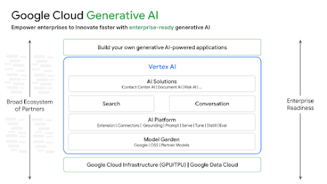
Vertex AI is a fully-managed, unified AI development platform for building and using generative AI. Access and utilize AI Studio, Agent Builder, and 130+ foundation models including Gemini 1.5 Pro—all from Vertex AI.
New customers get up to $300 in free credits to try Vertex AI and other Google Cloud products.
Features
Gemini, Google’s most capable multimodal models
Vertex AI offers access to Gemini models from Google. Gemini is capable of understanding virtually any input, combining different types of information, and generating almost any output. Prompt and test in Vertex AI with Gemini, using text, images, video, or code. Using Gemini’s advanced reasoning and state-of-the-art generation capabilities, developers can try sample prompts for extracting text from images, converting image text to JSON, and even generate answers about uploaded images to build next-gen AI applications.
In addition to Gemini, you also have access to Gemma, a family of lightweight, state-of-the-art open models built from the same research and technology used to create the Gemini models.
130+ generative AI models and tools
Choose from the widest variety of models with first-party (Gemini, Imagen, Codey), third-party (Anthropic's Claude 3), and open models (Gemma, Llama 2) in Model Garden. Use extensions to enable models to retrieve real-time information and trigger actions. Customize models to your use case with a variety of tuning options for Google's text, image, or code models.
Generative AI models and fully managed tools make it easy to prototype, customize, and integrate and deploy them into applications.
Open and integrated AI platform
Data scientists can move faster with Vertex AI Platform's tools for training, tuning, and deploying ML models.
Vertex AI notebooks, including your choice of Colab Enterprise or Workbench, are natively integrated with BigQuery providing a single surface across all data and AI workloads.
Vertex AI Training and Prediction help you reduce training time and deploy models to production easily with your choice of open source frameworks and optimized AI infrastructure.

MLOps for predictive and generative AI
Vertex AI Platform provides purpose-built MLOps tools for data scientists and ML engineers to automate, standardize, and manage ML projects.
Modular tools help you collaborate across teams and improve models throughout the entire development life cycle—identify the best model for a use case with Vertex AI Evaluation, orchestrate workflows with Vertex AI Pipelines, manage any model with Model Registry, serve, share, and reuse ML features with Feature Store, and monitor models for input skew and drift.
Agent Builder
Vertex AI Agent Builder enables developers to easily build and deploy enterprise ready generative AI experiences. It provides the convenience of a no code agent builder console alongside powerful grounding, orchestration and customization capabilities. With Vertex AI Agent Builder developers can quickly create a range of generative AI agents and applications grounded in their organization’s data.
AI solutions
Built on top of Vertex AI Platform, Contact Center AI, Document AI, Anti Money Laundering AI, Discovery AI, and other AI solutions provide powerful and targeted capabilities to enable specific business results. Businesses can access, deploy, and use Google Cloud's AI solutions directly, or supported by one of our priority partners.
How It Works
Built on Google’s AI research and powered by AI infrastructure, Vertex AI enables everyone to build and use AI with an open, responsible, and secure approach.
Common Uses
Build with Gemini
Access Gemini Pro via the Gemini API in Google Cloud Vertex AI
- Python
- JavaScript
- Java
- Go
- Curl
Code sample
Access Gemini Pro via the Gemini API in Google Cloud Vertex AI
- Python
- JavaScript
- Java
- Go
- Curl
Generative AI in applications
Get an introduction to generative AI on Vertex AI
Get an introduction to generative AI on Vertex AI
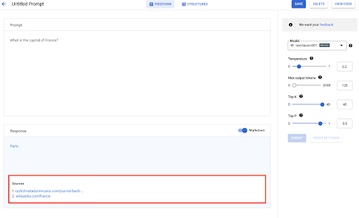
Vertex AI Studio offers a Google Cloud console tool for rapidly prototyping and testing generative AI models. Learn how you can use Generative AI Studio to test models using prompt samples, design and save prompts, tune a foundation model, and convert between speech and text.
See how to tune LLMs in Vertex AI Studio
Tutorials, quickstarts, & labs
Get an introduction to generative AI on Vertex AI
Get an introduction to generative AI on Vertex AI
Vertex AI Studio offers a Google Cloud console tool for rapidly prototyping and testing generative AI models. Learn how you can use Generative AI Studio to test models using prompt samples, design and save prompts, tune a foundation model, and convert between speech and text.
See how to tune LLMs in Vertex AI Studio
Extract, summarize, and classify data
Use gen AI for summarization, classification, and extraction
Use gen AI for summarization, classification, and extraction
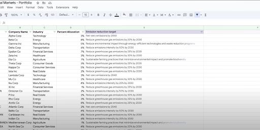
Learn how to create text prompts for handling any number of tasks with Vertex AI’s generative AI support. Some of the most common tasks are classification, summarization, and extraction. Vertex AI’s PaLM API for text lets you design prompts with flexibility in terms of their structure and format.
See how you can accelerate research and discovery with generative AI.
Tutorials, quickstarts, & labs
Use gen AI for summarization, classification, and extraction
Use gen AI for summarization, classification, and extraction
Learn how to create text prompts for handling any number of tasks with Vertex AI’s generative AI support. Some of the most common tasks are classification, summarization, and extraction. Vertex AI’s PaLM API for text lets you design prompts with flexibility in terms of their structure and format.
See how you can accelerate research and discovery with generative AI.
Train custom ML models
Custom ML training overview and documentation
Custom ML training overview and documentation
Get an overview of the custom training workflow in Vertex AI, the benefits of custom training, and the various training options that are available. This page also details every step involved in the ML training workflow from preparing data to predictions.
Get a video walkthrough of the steps required to train custom models on Vertex AI.
Tutorials, quickstarts, & labs
Custom ML training overview and documentation
Custom ML training overview and documentation
Get an overview of the custom training workflow in Vertex AI, the benefits of custom training, and the various training options that are available. This page also details every step involved in the ML training workflow from preparing data to predictions.
Get a video walkthrough of the steps required to train custom models on Vertex AI.
Train models with minimal ML expertise
Train and create ML models with minimal technical expertise
Train and create ML models with minimal technical expertise
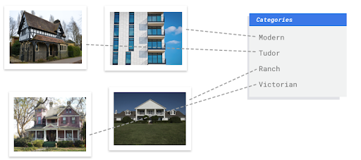
This guide walks you through how Vertex AI’s AutoML how to create and train high-quality custom machine learning models with minimal effort and machine learning expertise. This is perfect for those looking well to automate the tedious and time-consuming work of manually curating videos, images, texts, and tables.
Tutorials, quickstarts, & labs
Train and create ML models with minimal technical expertise
Train and create ML models with minimal technical expertise
This guide walks you through how Vertex AI’s AutoML how to create and train high-quality custom machine learning models with minimal effort and machine learning expertise. This is perfect for those looking well to automate the tedious and time-consuming work of manually curating videos, images, texts, and tables.
Deploy a model for production use
Deploy for batch or online predictions
Deploy for batch or online predictions
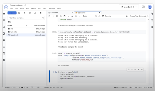
When you're ready to use your model to solve a real-world problem, register your model to Vertex AI Model Registry and use the Vertex AI prediction service for batch and online predictions.
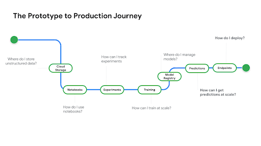
Watch Prototype to Production, a video series that takes you from notebook code to a deployed model.
Tutorials, quickstarts, & labs
Deploy for batch or online predictions
Deploy for batch or online predictions
When you're ready to use your model to solve a real-world problem, register your model to Vertex AI Model Registry and use the Vertex AI prediction service for batch and online predictions.
Watch Prototype to Production, a video series that takes you from notebook code to a deployed model.
Pricing
| How Vertex AI pricing works | Pricing is based on the Vertex AI tools and services, storage, compute, and Google Cloud resources used. | |
|---|---|---|
| Tools and usage | Description | Price |
Generative AI | Imagen model for image generation Based on image input, character input, or custom training pricing. | Starting at $0.0001 |
Text, chat, and code generation Based on every 1,000 characters of input (prompt) and every 1,000 characters of output (response). | Starting at $0.0001 per 1,000 characters | |
AutoML models | Image data training, deployment, and prediction Based on time to train per node hour, which reflects resource usage, and if for classification or object detection. | Starting at $1.375 per node hour |
Video data training and prediction Based on price per node hour and if classification, object tracking, or action recognition. | Starting at $0.462 per node hour | |
Tabular data training and prediction Based on price per node hour and if classification/regression or forecasting. Contact sales for potential discounts and pricing details. | Contact sales | |
Text data upload, training, deployment, prediction Based on hourly rates for training and prediction, pages for legacy data upload (PDF only), and text records and pages for prediction. | Starting at $0.05 per hour | |
Custom-trained models | Custom model training Based on machine type used per hour, region, and any accelerators used. Get an estimate via sales or our pricing calculator. | Contact sales |
Vertex AI notebooks | Compute and storage resources Based on the same rates as Compute Engine and Cloud Storage. | Refer to products |
Management fees In addition to the above resource usage, management fees apply based on region, instances, notebooks, and managed notebooks used. View details. | Refer to details | |
Vertex AI Pipelines | Execution and additional fees Based on execution charge, resources used, and any additional service fees. | Starting at $0.03 per pipeline run |
Vertex AI Vector Search | Serving and building costs Based on the size of your data, the amount of queries per second (QPS) you want to run, and the number of nodes you use. View example. | Refer to example |
View pricing details for all Vertex AI features and services.
How Vertex AI pricing works
Pricing is based on the Vertex AI tools and services, storage, compute, and Google Cloud resources used.
Generative AI
Imagen model for image generation
Based on image input, character input, or custom training pricing.
Starting at
$0.0001
Text, chat, and code generation
Based on every 1,000 characters of input (prompt) and every 1,000 characters of output (response).
Starting at
$0.0001
per 1,000 characters
AutoML models
Image data training, deployment, and prediction
Based on time to train per node hour, which reflects resource usage, and if for classification or object detection.
Starting at
$1.375
per node hour
Video data training and prediction
Based on price per node hour and if classification, object tracking, or action recognition.
Starting at
$0.462
per node hour
Tabular data training and prediction
Based on price per node hour and if classification/regression or forecasting. Contact sales for potential discounts and pricing details.
Contact sales
Text data upload, training, deployment, prediction
Based on hourly rates for training and prediction, pages for legacy data upload (PDF only), and text records and pages for prediction.
Starting at
$0.05
per hour
Custom-trained models
Custom model training
Based on machine type used per hour, region, and any accelerators used. Get an estimate via sales or our pricing calculator.
Contact sales
Vertex AI notebooks
Refer to products
Management fees
In addition to the above resource usage, management fees apply based on region, instances, notebooks, and managed notebooks used. View details.
Refer to details
Vertex AI Pipelines
Execution and additional fees
Based on execution charge, resources used, and any additional service fees.
Starting at
$0.03
per pipeline run
Vertex AI Vector Search
Serving and building costs
Based on the size of your data, the amount of queries per second (QPS) you want to run, and the number of nodes you use. View example.
Refer to example
View pricing details for all Vertex AI features and services.
Pricing calculator
Custom quote
Start your proof of concept
New customers get up to $300 in free credits to try Vertex AI and other Google Cloud products
Have a large project?
Browse, customize, and deploy machine learning models
Learn how to set up a Vertex AI project environment
Get started with notebooks for machine learning
FAQ
What is Vertex AI used for?
Vertex AI helps anyone in your organization benefit from AI/ML—from business users working with Vertex AI solutions to developers building generative AI applications with Vertex AI Agent Builder, to data scientists and ML engineers who can train and deploy ML models efficiently.
Why use Vertex AI Platform?
Vertex AI Platform unifies the entire ML workflow from training to deployment, and can help organizations accelerate AI production, including with generative AI models, and has a high recommendation rate on Gartner Peer Insights.
Is Google Cloud's Vertex AI free?
New customers get $300 in free credits to spend on Vertex AI when they sign up for the free trial.
How do I get access to Gemini models in Vertex AI?
Gemini 1.0 Pro, our best model for scaling across AI tasks, is now generally available to all Vertex AI customers. 1.0 Pro offers the best balance of quality, performance, and cost for most AI tasks, like content generation, editing, summarization, and classification. Try Gemini in Vertex AI
Gemini 1.0 Ultra, our most sophisticated and capable model for complex tasks, is now generally available on Vertex AI for customers via allowlist. 1.0 Ultra is designed for complex tasks, showing especially strong performance in areas such as complex instruction, code, reasoning, and multilinguality, and is optimized for high quality output. For access contact your Google Cloud account rep.


