이 둘러보기에는 Apache Beam, Google Dataflow, TensorFlow를 사용하여 머신러닝 모델을 사전 처리하고, 학습시키고, 예측하는 방법을 보여줍니다.
이러한 개념을 설명하기 위해 이 둘러보기에서는 분자 코드 샘플을 사용합니다. 분자 코드 샘플은 주어진 분자 데이터를 입력값으로 하여 머신러닝 모델을 생성하고 학습하여 분자 에너지를 예측합니다.
비용
이 둘러보기에서는 다음 중 하나 이상을 포함하고 비용이 청구될 수 있는 Google Cloud 구성요소를 사용할 가능성이 있습니다.
- Dataflow
- Cloud Storage
- AI Platform
가격 계산기를 사용하여 예상 사용량을 토대로 예상 비용을 산출할 수 있습니다.
개요
분자 코드 샘플은 분자 데이터가 포함된 파일을 추출하며 각 분자에 있는 탄소, 수소, 산소, 질소 원자의 수를 계산합니다. 그런 다음 해당 수를 0과 1 사이의 값으로 정규화하고 TensorFlow 심층신경망 에스티메이터로 전달합니다. 신경망 에스티메이터는 머신러닝 모델을 학습시켜 분자 에너지를 예측합니다.
코드 샘플은 다음과 같은 4가지 단계로 구성됩니다.
- 데이터 추출(
data-extractor.py) - 사전 처리(
preprocess.py) - 학습(
trainer/task.py) - 예측(
predict.py)
아래의 섹션에서는 4가지 단계를 살펴보지만 이 둘러보기에서는 Apache Beam과 Dataflow를 사용하는 단계인 사전 처리 단계와 예측 단계에 중점을 둡니다. 사전 처리 단계에서는 TensorFlow 변환 라이브러리(일반적으로 tf.Transform)도 사용합니다.
다음 이미지는 분자 코드 샘플의 워크플로를 보여줍니다.

코드 샘플 실행
환경을 설정하려면 분자 GitHub 저장소의 README에 있는 안내를 따릅니다. 그런 다음 제공된 래퍼 스크립트 run-local 또는 run-cloud 중 하나를 사용해 분자 코드 샘플을 실행합니다. 이 스크립트는 4가지 코드 샘플 단계(추출, 사전 처리, 학습, 예측)를 모두 자동으로 실행합니다.
또는 이 문서의 섹션에 제공된 명령어를 사용하여 수동으로 각 단계를 실행할 수 있습니다.
로컬에서 실행
분자 코드 샘플을 로컬에서 실행하려면 run-local 래퍼 스크립트를 실행합니다.
./run-local
출력 로그는 스크립트가 4가지 단계(데이터 추출, 사전 처리, 학습, 예측)를 각각 실행하는 시기를 보여줍니다.
data-extractor.py 스크립트에는 파일 수에 필요한 필수 인수가 있습니다.
쉽게 사용할 수 있도록 run-local 스크립트 및 run-cloud 스크립트는 이 인수에 대해 기본적으로 5개 파일이 있습니다. 각 파일에는 25,000개의 분자가 포함되어 있습니다. 코드 샘플을 처음부터 끝까지 실행하는 데에는 약 3~7분이 소요됩니다. 실행 시간은 컴퓨터의 CPU에 따라 달라집니다.
Google Cloud에서 실행
Google Cloud에서 분자 코드 샘플을 실행하려면 run-cloud 래퍼 스크립트를 실행합니다. 입력 파일은 모두 Cloud Storage에 있어야 합니다.
--work-dir 매개변수를 Cloud Storage 버킷으로 설정합니다.
./run-cloud --work-dir gs://<your-bucket-name>/cloudml-samples/molecules
1단계: 데이터 추출
소스 코드: data-extractor.py
첫 번째 단계는 입력 데이터를 추출하는 것입니다. data-extractor.py 파일은 지정된 SDF 파일을 추출하여 압축을 해제합니다. 이후 단계의 예시에서는 이러한 파일을 사전 처리하고 데이터를 사용하여 머신러닝 모델을 학습하고 평가합니다. 이 파일은 공개 소스에서 SDF 파일을 추출하여 지정된 작업 디렉터리 내에 있는 하위 디렉터리에 저장합니다. 기본 작업 디렉터리(--work-dir)는 /tmp/cloudml-samples/molecules입니다.
추출된 파일 저장
추출된 데이터 파일을 로컬에 저장합니다.
python data-extractor.py --max-data-files 5
또는 추출된 데이터 파일을 Cloud Storage 위치에 저장합니다.
WORK_DIR=gs://<your bucket name>/cloudml-samples/molecules

python data-extractor.py --work-dir $WORK_DIR --max-data-files 5
2단계: 사전 처리
소스 코드: preprocess.py
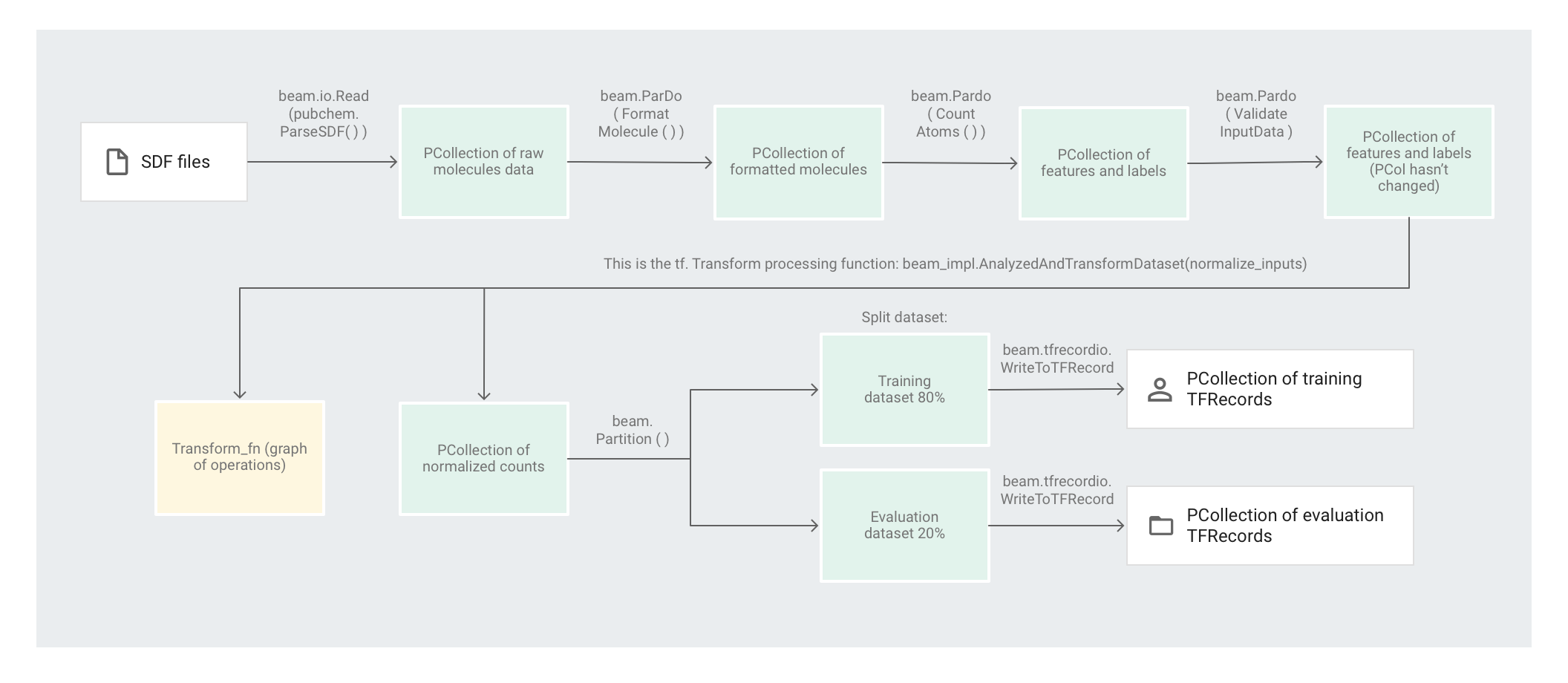
분자 코드 샘플에서는 Apache Beam 파이프라인을 사용하여 데이터를 사전 처리합니다. 이 파이프라인은 다음과 같은 사전 처리 작업을 이행합니다.
- 추출된 SDF 파일을 읽고 파싱합니다.
- 파일의 각 분자에 있는 다양한 원자의 수를 계산합니다.
tf.Transform을 사용하여 개수를 0에서 1 사이의 값으로 정규화합니다.- 데이터 세트를 학습 데이터 세트와 평가 데이터 세트로 파티션을 나눕니다.
- 두 데이터 세트를
TFRecord객체로 작성합니다.
Apache Beam 변환은 한 번에 요소 하나를 효율적으로 조작할 수 있지만, 데이터 세트의 전체 전달이 필요한 변환의 경우에는 Apache Beam만으로는 쉽게 조작할 수 없으며 tf.Transform을 사용하면 쉽게 조작할 수 있습니다. 이 때문에 코드에서는 Apache Beam 변환을 사용하여 분자를 읽고 형식을 지정하며 각 분자의 원자 수를 계산합니다. 그런 다음 코드는 데이터를 정규화하기 위해 tf.Transform을 사용하여 전역 최소 및 최대 개수를 찾습니다.
다음 이미지는 파이프라인의 단계를 보여줍니다.
요소 기반 변환 적용
preprocess.py 코드는 Apache Beam 파이프라인을 생성합니다.
그런 다음 코드는 파이프라인에 feature_extraction 변환을 적용합니다.
파이프라인에서는 SimpleFeatureExtraction을 feature_extraction 변환으로 사용합니다.
pubchem/pipeline.py에서 정의된 SimpleFeatureExtraction 변환에는 모든 요소를 독립적으로 조작하는 일련의 변환이 포함되어 있습니다.
먼저 코드는 소스 파일에서 분자를 파싱하고, 분자 속성의 사전으로 분자의 형식을 지정한 다음 마지막으로 분자에 있는 원자 수를 계산합니다. 이 숫자는 머신러닝 모델의 특징(입력)입니다.
읽기 변환 beam.io.Read(pubchem.ParseSDF(data_files_pattern))는 커스텀 소스에서 SDF 파일을 읽습니다.
ParseSDF라는 커스텀 소스는 pubchem/pipeline.py에 정의되어 있습니다.
ParseSDF는 FileBasedSource를 확장하고 추출된 SDF 파일을 여는 read_records 함수를 구현합니다.
Google Cloud에서 분자 코드 샘플을 실행하면 여러 작업자(VM)가 동시에 파일을 읽을 수 있습니다. 두 작업자가 파일의 동일한 콘텐츠를 읽지 않도록 하려면 각 파일에서 range_tracker를 사용합니다.
파이프라인은 원시 데이터를 다음 단계에 필요한 관련 정보 섹션으로 그룹화합니다. 파싱된 SDF 파일의 각 섹션은 사전(pipeline/sdf.py 참조)에 저장됩니다. 여기서 키는 섹션 이름이고 값은 해당 섹션의 원시 라인 콘텐츠입니다.
코드는 파이프라인에 beam.ParDo(FormatMolecule())을 적용합니다. ParDo는 각 분자에 이름이 FormatMolecule인 DoFn을 적용합니다. FormatMolecule은 형식이 지정된 분자의 사전을 생성합니다. 다음 스니펫은 출력 PCollection의 요소 예시입니다.
{
  'atoms': [
    {
      'atom_atom_mapping_number': 0,
      'atom_stereo_parity': 0,
      'atom_symbol': u'O',
      'charge': 0,
      'exact_change_flag': 0,
      'h0_designator': 0,
      'hydrogen_count': 0,
      'inversion_retention': 0,
      'mass_difference': 0,
      'stereo_care_box': 0,
      'valence': 0,
      'x': -0.0782,
      'y': -1.5651,
      'z': 1.3894,
    },
    ...
  ],
  'bonds': [
    {
      'bond_stereo': 0,
      'bond_topology': 0,
      'bond_type': 1,
      'first_atom_number': 1,
      'reacting_center_status': 0,
      'second_atom_number': 5,
    },
    ...
  ],
  '<PUBCHEM_COMPOUND_CID>': ['3\n'],
  ...
  '<PUBCHEM_MMFF94_ENERGY>': ['19.4085\n'],
  ...
}
그런 다음 코드는 파이프라인에 beam.ParDo(CountAtoms())를 적용합니다. DoFn CountAtoms는 각 분자에 있는 탄소, 수소, 질소, 산소 원자의 수를 합산합니다. CountAtoms는 특징 및 라벨의 PCollection을 출력합니다.
다음은 출력 PCollection의 요소 예시입니다.
{
  'ID': 3,
  'TotalC': 7,
  'TotalH': 8,
  'TotalO': 4,
  'TotalN': 0,
  'Energy': 19.4085,
}
그런 다음 파이프라인은 입력을 검증합니다. ValidateInputData DoFn은 모든 요소가 input_schema에 제공된 메타데이터와 일치하는지 확인합니다. 이러한 유효성 검사를 통해 데이터가 TensorFlow로 전달할 때 올바른 형식인지 확인합니다.
전체 전달 변환 적용
분자 코드 샘플은 심층신경망 회귀자를 사용하여 예측합니다. 일반적으로 입력을 정규화한 다음 ML 모델로 전달하는 것이 좋습니다. 파이프라인은 tf.Transform을 사용하여 각 원자의 수를 0과 1 사이의 값으로 정규화합니다. 입력 정규화에 대한 자세한 내용은 특징 확장을 참조하세요.
값을 정규화하려면 데이터 세트를 전체 전달하여 최솟값과 최댓값을 기록해야 합니다. 코드는 tf.Transform을 사용하여 전체 데이터 세트를 살펴보고 전체 전달 변환을 적용합니다.
tf.Transform을 사용하려면 데이터 세트에서 수행할 변환의 논리가 포함된 함수를 코드에서 제공해야 합니다. preprocess.py에서 코드는 tf.Transform에서 제공하는 AnalyzeAndTransformDataset 변환을 사용합니다. tf.Transform 사용 방법에 대해 자세히 알아보세요.
preprocess.py에서 사용된 feature_scaling 함수는 pubchem/pipeline.py에 정의된 normalize_inputs입니다. 이 함수는 tf.Transform 함수 scale_to_0_1를 사용하여 수를 0에서 1 사이의 값으로 정규화합니다.
데이터를 수동으로 정규화할 수도 있지만 데이터 세트가 클 경우 Dataflow를 사용하는 것이 더 빠릅니다. Dataflow를 사용하면 필요에 따라 파이프라인을 여러 작업자(VM)에서 실행할 수 있습니다.
데이터 세트 파티션 나누기
다음으로 preprocess.py 파이프라인은 데이터 세트 하나를 2개의 데이터 세트로 파티션을 나눕니다. 데이터의 약 80%를 학습 데이터로 사용하고 데이터의 약 20%를 평가 데이터로 사용하도록 할당합니다.
출력 작성
마지막으로 preprocess.py 파이프라인은 WriteToTFRecord 변환을 사용하여 두 개의 데이터 세트(학습 및 평가)를 작성합니다.
사전 처리 파이프라인 실행
사전 처리 파이프라인을 로컬에서 실행합니다.
python preprocess.py
또는 사전 처리 파이프라인을 Dataflow에서 실행합니다.
PROJECT=$(gcloud config get-value project)
WORK_DIR=gs://<your bucket name>/cloudml-samples/molecules
python preprocess.py \
  --project $PROJECT \
  --runner DataflowRunner \
  --temp_location $WORK_DIR/beam-temp \
  --setup_file ./setup.py \
  --work-dir $WORK_DIR
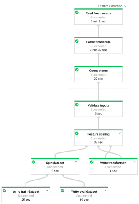
파이프라인을 실행한 후에는 Dataflow 모니터링 인터페이스에서 파이프라인의 진행 상황을 볼 수 있습니다.
3단계: 학습
소스 코드: trainer/task.py
사전 처리 단계가 끝날 때 코드는 두 개의 데이터 세트(학습 및 평가)로 데이터를 분할합니다.
이 샘플은 TensorFlow를 사용하여 머신러닝 모델을 학습합니다. 분자 코드 샘플의 trainer/task.py 파일에는 모델을 학습하기 위한 코드가 포함되어 있습니다. trainer/task.py의 기본 함수는 사전 처리 단계에서 처리된 데이터를 로드합니다.
에스티메이터는 학습 데이터 세트를 사용하여 모델을 학습한 다음 평가 데이터 세트를 사용하여 모델이 일부 분자 속성에 따라 분자 에너지를 정확하게 예측하는지 확인합니다.
ML 모델 학습에 대해 자세히 알아보세요.
모델 학습
로컬에서 모델을 학습합니다.
python trainer/task.py

# To get the path of the trained model
EXPORT_DIR=/tmp/cloudml-samples/molecules/model/export/final
MODEL_DIR=$(ls -d -1 $EXPORT_DIR/* | sort -r | head -n 1)
또는 AI Platform에서 모델을 학습시킵니다.
- 먼저 지원되는 리전을 선택하여 학습 작업을 실행합니다.
gcloud config set compute/region $REGION
- 학습 작업을 실행합니다.
JOB="cloudml_samples_molecules_$(date +%Y%m%d_%H%M%S)"
BUCKET=gs://<your bucket name>
WORK_DIR=$BUCKET/cloudml-samples/molecules
gcloud ai-platform jobs submit training $JOB \
  --module-name trainer.task \
  --package-path trainer \
  --staging-bucket $BUCKET \
  --runtime-version 1.13 \
  --stream-logs \
  -- \
  --work-dir $WORK_DIR

# To get the path of the trained model:
EXPORT_DIR=$WORK_DIR/model/export
MODEL_DIR=$(gsutil ls -d $EXPORT_DIR/* | sort -r | head -n 1)
4단계: 예측
소스 코드: predict.py
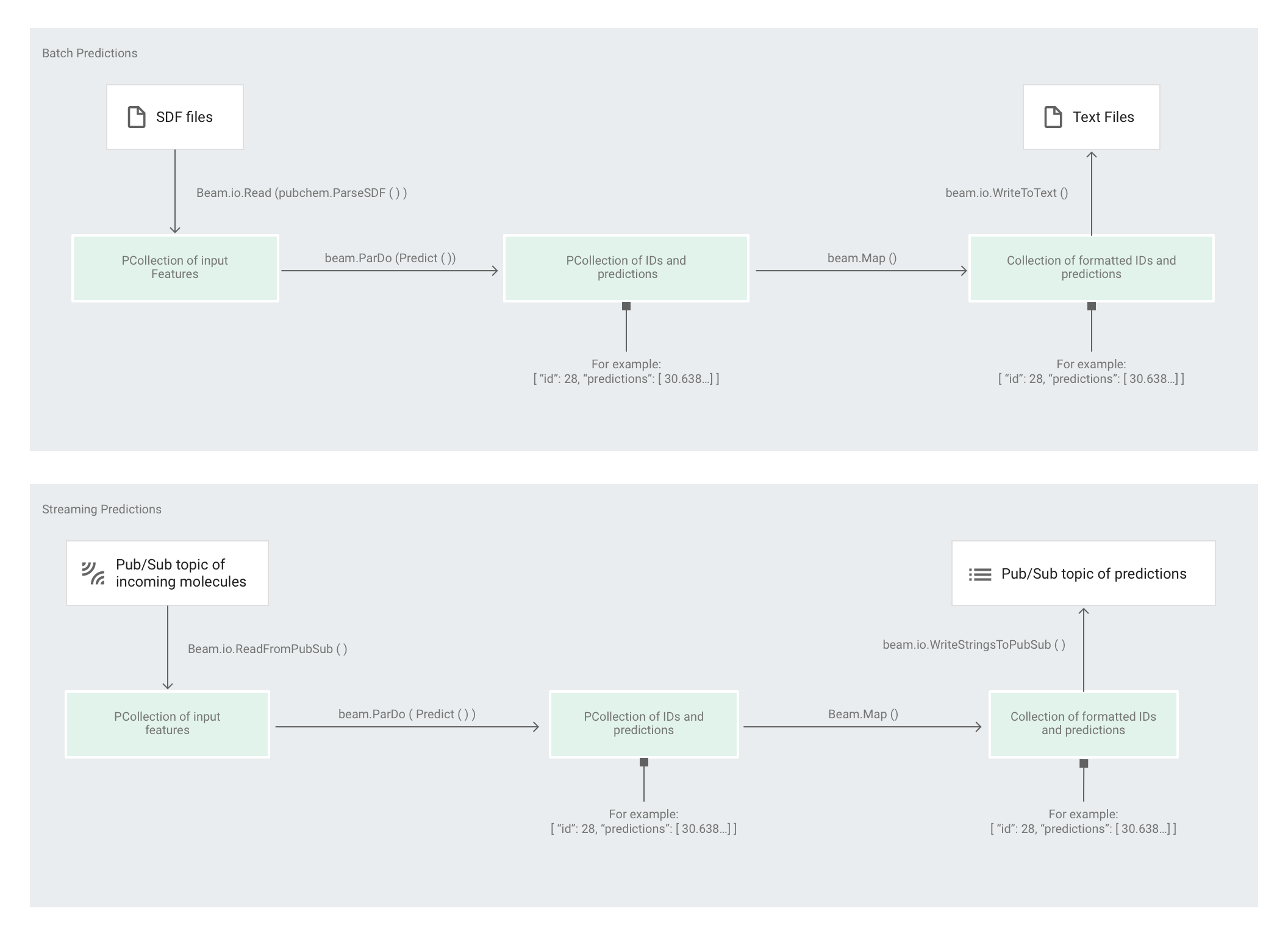
에스티메이터에서 모델을 학습한 후에는 모델에 입력을 제공할 수 있으며 이 경우 모델에서 예측을 수행합니다. 분자 코드 샘플에서는 predict.py의 파이프라인이 예측을 담당합니다. 이 파이프라인은 배치 파이프라인 또는 스트리밍 파이프라인의 역할을 할 수 있습니다.
파이프라인의 코드는 소스와 싱크 상호작용을 제외하고 배치와 스트리밍에서 동일합니다. 파이프라인이 배치 모드에서 실행되는 경우 커스텀 소스에서 입력 파일을 읽고 출력 예측을 텍스트 파일로 지정된 작업 디렉터리에 작성합니다. 파이프라인이 스트리밍 모드에서 실행되는 경우 입력 분자가 도착할 때 Pub/Sub 주제에서 읽습니다. 파이프라인은 준비된 경우 다른 Pub/Sub 주제에 출력 예측을 작성합니다.
다음 이미지는 예측 파이프라인(배치 및 스트리밍)의 단계를 보여줍니다.
predict.py에서 코드는 run 함수에서 파이프라인을 정의합니다.
코드는 다음 매개변수를 사용하여 run 함수를 호출합니다.
먼저 코드는 pubchem.SimpleFeatureExtraction(source) 변환을 feature_extraction 변환으로 전달합니다. 사전 처리 단계에서도 사용된 이러한 변환은 파이프라인에 적용됩니다.
변환은 파이프라인의 실행 모드(배치 또는 스트리밍)를 기반으로 적절한 소스에서 읽고, 분자의 형식을 지정하고, 각 분자에 있는 다양한 원자의 수를 계산합니다.
다음으로 beam.ParDo(Predict(…))가 분자 에너지를 예측하는 파이프라인에 적용됩니다.
전달된 DoFn인 Predict는 지정된 입력 특징(원자 개수)의 사전을 사용하여 분자 에너지를 예측합니다.
파이프라인에 적용되는 다음 변환은 beam.Map(lambda result: json.dumps(result))입니다. 이 변환은 예측 결과 사전을 가져와 JSON 문자열로 직렬화합니다.
마지막으로 싱크에 출력이 작성됩니다(일괄 모드인 경우 텍스트 파일로 작업 디렉터리에 작성되며, 스트리밍 모드인 경우 메시지로 Pub/Sub 주제에 게시됨).
일괄 예측
배치 예측은 지연 시간이 아닌 처리량에 따라 최적화됩니다. 배치 예측은 여러 번을 예측하고 모든 예측을 완료하여 결과를 얻을 때까지 기다릴 수 있는 경우에 가장 효과적입니다.
배치 모드에서 예측 파이프라인 실행
일괄 예측 파이프라인을 로컬에서 실행합니다.
# For simplicity, we'll use the same files we used for training
python predict.py \
  --model-dir $MODEL_DIR \
  batch \
  --inputs-dir /tmp/cloudml-samples/molecules/data \
  --outputs-dir /tmp/cloudml-samples/molecules/predictions
또는 일괄 예측 파이프라인을 Dataflow에서 실행합니다.
# For simplicity, we'll use the same files we used for training
PROJECT=$(gcloud config get-value project)
WORK_DIR=gs://<your bucket name>/cloudml-samples/molecules
python predict.py \
  --work-dir $WORK_DIR \
  --model-dir $MODEL_DIR \
  batch \
  --project $PROJECT \
  --runner DataflowRunner \
  --temp_location $WORK_DIR/beam-temp \
  --setup_file ./setup.py \
  --inputs-dir $WORK_DIR/data \
  --outputs-dir $WORK_DIR/predictions
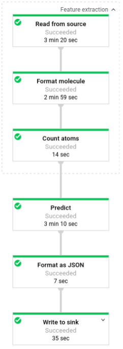
파이프라인을 실행한 후에는 Dataflow 모니터링 인터페이스에서 파이프라인의 진행 상황을 볼 수 있습니다.
스트리밍 예측
스트리밍 예측은 처리량이 아닌 지연 시간에 따라 최적화됩니다. 스트리밍 예측은 산발적으로 예측하지만 가능한 한 빨리 결과를 얻으려고 할 경우 가장 효과적입니다.
예측 서비스(스트리밍 예측 파이프라인)는 Pub/Sub 주제에서 입력 분자를 받고 다른 Pub/Sub 주제에 출력(예측)을 게시합니다.
입력 Pub/Sub 주제를 만듭니다.
gcloud pubsub topics create molecules-inputs
출력 Pub/Sub 주제를 만듭니다.
gcloud pubsub topics create molecules-predictions
스트리밍 예측 파이프라인을 로컬에서 실행합니다.
# Run on terminal 1
PROJECT=$(gcloud config get-value project)
python predict.py \
  --model-dir $MODEL_DIR \
  stream \
  --project $PROJECT
  --inputs-topic molecules-inputs \
  --outputs-topic molecules-predictions
또는 Dataflow에서 스트리밍 예측 파이프라인을 실행합니다.
# Run on terminal 1
PROJECT=$(gcloud config get-value project)
WORK_DIR=gs://<your bucket name>/cloudml-samples/molecules
python predict.py \
  --work-dir $WORK_DIR \
  --model-dir $MODEL_DIR \
  stream \
  --project $PROJECT
  --runner DataflowRunner \
  --temp_location $WORK_DIR/beam-temp \
  --setup_file ./setup.py \
  --inputs-topic molecules-inputs \
  --outputs-topic molecules-predictions
예측 서비스(스트리밍 예측 파이프라인)를 실행한 후에는 게시자를 실행하여 분자를 예측 서비스에 보내고 구독자를 실행하여 예측 결과를 리슨해야 합니다. 분자 코드 샘플은 게시자(publisher.py)와 구독자(subscriber.py) 서비스를 제공합니다.
게시자는 디렉터리에서 SDF 파일을 파싱하여 입력 주제에 게시합니다. 구독자는 예측 결과를 수신하고 로깅합니다. 쉽게 설명하기 위해 이 예시에서는 학습 단계에 사용된 것과 동일한 SDF 파일을 사용합니다.
구독자를 실행합니다.
# Run on terminal 2
python subscriber.py \
  --project $PROJECT \
  --topic molecules-predictions
게시자를 실행합니다.
# Run on terminal 3
python publisher.py \
  --project $PROJECT \
  --topic molecules-inputs \
  --inputs-dir $WORK_DIR/data
게시자가 분자 파싱과 게시를 시작하면 구독자에서 예측을 볼 수 있습니다.
삭제
스트리밍 예측 파이프라인 실행을 완료한 후에는 요금이 부과되지 않도록 파이프라인을 중지하세요.
다음 단계
- Apache Beam 문서 참조
- TensorFlow 문서 읽어보기:
- Apache Beam 및
tf.Transform을 사용하는 다른 코드 샘플 사용해 보기 - Global Fishing Watch 예시를 사용하여 시계열 분류에 사용되는 ML 모델 학습