本演示介绍了如何使用 Apache Beam、Google Dataflow 和 TensorFlow 对机器学习模型进行预处理、训练和执行预测。
本演示使用分子代码示例来演示这些概念。 分子代码示例会将分子数据作为输入,创建并训练机器学习模型来预测分子能量。
费用
本演示可能会使用 Google Cloud 的一项或多项收费组件,包括:
- Dataflow
- Cloud Storage
- AI Platform
请使用价格计算器根据您的预计用量来估算费用。
概览
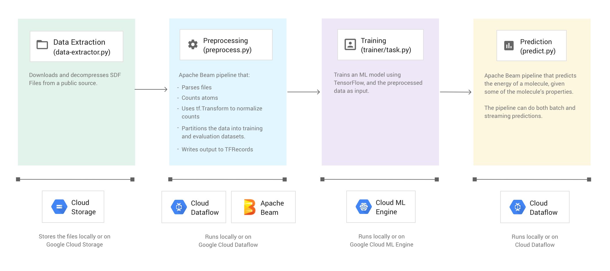
分子代码示例会提取包含分子数据的文件,并计算每个分子中所含的碳原子、氢原子、氧原子和氮原子的数量。 然后,该代码会将各计数归一化为 0 到 1 之间的值,并将这些值馈送到 TensorFlow 深度神经网络 Estimator。神经网络 Estimator 会训练机器学习模型来预测分子能量。
代码示例包含以下四个阶段:
- 数据提取 (
data-extractor.py) - 预处理 (
preprocess.py) - 训练 (
trainer/task.py) - 预测 (
predict.py)
以下部分逐步介绍了这四个阶段,不过,本演示重点介绍的是使用 Apache Beam 和 Dataflow 的阶段,即预处理阶段和预测阶段。预处理阶段还会使用 TensorFlow Transform 库(通常称为 tf.Transform)。
下图显示了分子代码示例的工作流。
运行代码示例
请按照分子 GitHub 存储库的 README 中的说明设置您的环境。然后,使用提供的其中一个封装容器脚本(run-local 或 run-cloud)运行分子代码示例。这些脚本会自动运行代码示例的所有四个阶段(提取、预处理、训练和预测)。
或者,您也可以使用本文档各部分中提供的命令手动运行各个阶段。
在本地运行
要在本地运行分子代码示例,请运行 run-local 封装容器脚本:
./run-local
输出日志会显示该脚本运行这四个阶段(数据提取、预处理、训练和预测)的时间。
data-extractor.py 脚本有一个用于指定文件数量的必需参数。为便于使用,在 run-local 脚本和 run-cloud 脚本中,该参数均默认为 5 个文件。每个文件包含 25000 个分子。运行代码示例从开始到结束大约需要 3 至 7 分钟。运行时间会因计算机的 CPU 而有所不同。
在 Google Cloud 上运行
要在 Google Cloud 上运行分子代码示例,请运行 run-cloud 封装容器脚本。所有输入文件都必须位于 Cloud Storage 中。
请将 --work-dir 参数设置为 Cloud Storage 存储分区:
./run-cloud --work-dir gs://<your-bucket-name>/cloudml-samples/molecules
第 1 阶段:数据提取
第一步是提取输入数据。data-extractor.py 文件会提取并解压缩指定的 SDF 文件。在后续步骤中,该示例会预处理这些文件,并使用这些数据来训练和评估机器学习模型。该文件会从公共来源中提取 SDF 文件,并将它们存储在指定工作目录内的一个子目录中。默认工作目录 (--work-dir) 是 /tmp/cloudml-samples/molecules。
存储提取的文件
在本地存储提取的数据文件:
python data-extractor.py --max-data-files 5
或者,在 Cloud Storage 位置存储提取的数据文件:
WORK_DIR=gs://<your bucket name>/cloudml-samples/molecules

python data-extractor.py --work-dir $WORK_DIR --max-data-files 5
第 2 阶段:预处理
源代码:preprocess.py
分子代码示例使用 Apache Beam 流水线来预处理数据。 该流水线执行以下预处理操作:
- 读取并解析提取的 SDF 文件。
- 计算这些文件中各分子包含的不同原子数。
- 使用
tf.Transform将各计数归一化为 0 到 1 之间的值。 - 将数据集划分为训练数据集和评估数据集。
- 将两个数据集作为
TFRecord对象写入。
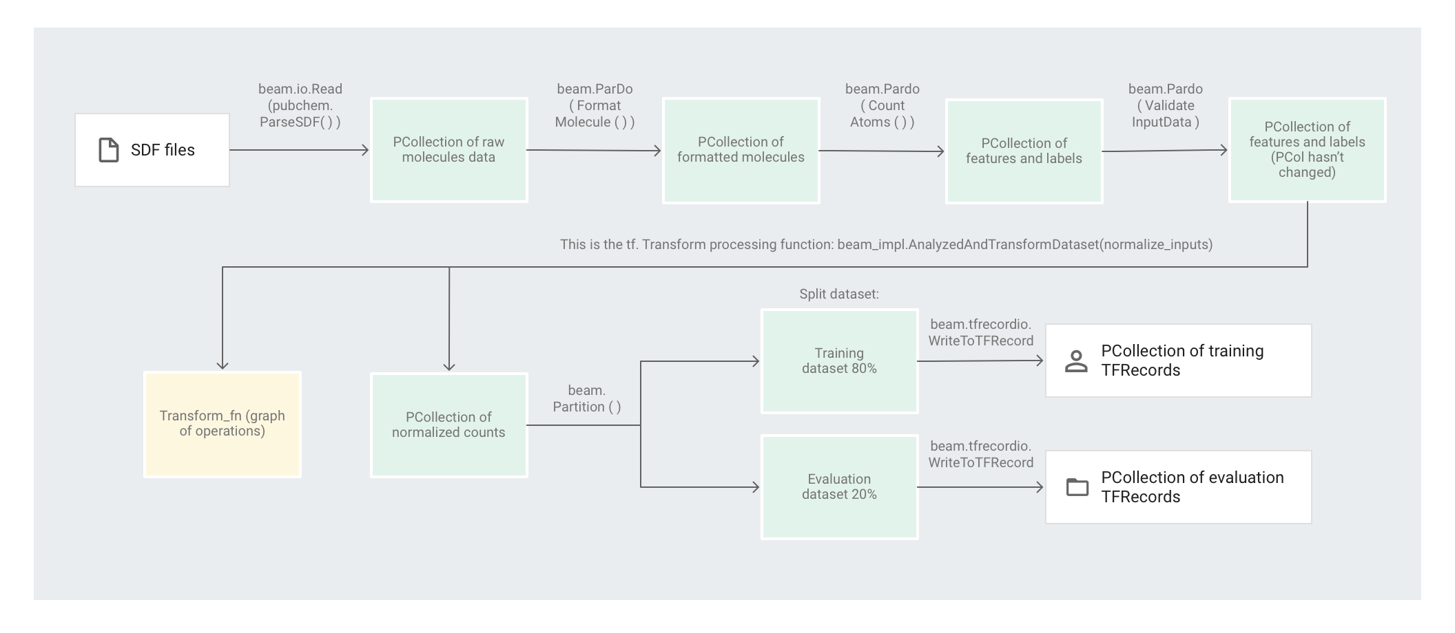
Apache Beam 转换一次可以有效操作单个元素,但需要对数据集进行全集扫描的转换无法单靠 Apache Beam 就轻松完成,最好是使用 tf.Transform 来执行。鉴于此,代码会先使用 Apache Beam 转换来读取分子、设置分子格式,并计算每个分子中的原子数量。然后,代码会使用 tf.Transform 来计算全局最小和最大计数,以便将数据归一化。
下图显示了此流水线中的各个步骤。
应用基于元素的转换
preprocess.py 代码会创建 Apache Beam 流水线。
然后,代码会将 feature_extraction 转换应用于该流水线。
该流水线使用 SimpleFeatureExtraction 作为其 feature_extraction 转换。
在 pubchem/pipeline.py 中定义的 SimpleFeatureExtraction 转换包含一系列转换,这些转换可独立操作所有元素。代码首先会解析源文件中的分子,接着将分子格式设置为分子属性字典,最后计算分子中的原子数量。这些计数是机器学习模型的特征(输入)。
读取转换 beam.io.Read(pubchem.ParseSDF(data_files_pattern)) 会从自定义来源读取 SDF 文件。
自定义来源名为 ParseSDF,在 pubchem/pipeline.py 中进行定义。ParseSDF 会扩展 FileBasedSource,并实现 read_records 函数来打开提取的 SDF 文件。
在 Google Cloud 上运行分子代码示例时,多个工作器(虚拟机)可以同时读取文件。为确保不会有两个工作器读取文件中的相同内容,每个文件都会使用 range_tracker。
该流水线会按后续步骤所需信息的相关性将原始数据划分为多个部分。解析后 SDF 文件中的每个部分会存储在字典中(请参阅 pipeline/sdf.py),其中键是部分名称,值是相应部分的原始行内容。
代码会将 beam.ParDo(FormatMolecule()) 应用于该流水线。ParDo 会将名为 FormatMolecule 的 DoFn 应用于每个分子。FormatMolecule 会生成一个由带格式分子构成的字典。以下代码段是输出 PCollection 中的一个元素示例:
{
  'atoms': [
    {
      'atom_atom_mapping_number': 0,
      'atom_stereo_parity': 0,
      'atom_symbol': u'O',
      'charge': 0,
      'exact_change_flag': 0,
      'h0_designator': 0,
      'hydrogen_count': 0,
      'inversion_retention': 0,
      'mass_difference': 0,
      'stereo_care_box': 0,
      'valence': 0,
      'x': -0.0782,
      'y': -1.5651,
      'z': 1.3894,
    },
    ...
  ],
  'bonds': [
    {
      'bond_stereo': 0,
      'bond_topology': 0,
      'bond_type': 1,
      'first_atom_number': 1,
      'reacting_center_status': 0,
      'second_atom_number': 5,
    },
    ...
  ],
  '<PUBCHEM_COMPOUND_CID>': ['3\n'],
  ...
  '<PUBCHEM_MMFF94_ENERGY>': ['19.4085\n'],
  ...
}
然后,代码会将 beam.ParDo(CountAtoms()) 应用于该流水线。DoFn CountAtoms 会对每个分子包含的碳原子、氢原子、氮原子和氧原子的数量求和。CountAtoms 会输出一个由特征和标签组成的 PCollection。
下面是输出 PCollection 中的一个元素示例:
{
  'ID': 3,
  'TotalC': 7,
  'TotalH': 8,
  'TotalO': 4,
  'TotalN': 0,
  'Energy': 19.4085,
}
该流水线随后会对输入进行验证。ValidateInputData DoFn 会验证每个元素是否与 input_schema 中指定的元数据匹配。此验证可确保数据馈入 TensorFlow 时采用正确的格式。
应用全集转换
分子代码示例使用深度神经网络回归器进行预测。一般情况下,建议先将输入归一化,然后再将其馈入机器学习模型。该流水线使用 tf.Transform 将各个原子数归一化为 0 到 1 之间的值。如需详细了解如何将输入归一化,请参阅特征缩放。
将值归一化需要对数据集进行全集扫描,并记录最小值和最大值。代码会使用 tf.Transform 对整个数据集进行全集扫描并应用全集转换。
要使用 tf.Transform,代码必须提供一个包含数据集转换逻辑的函数。在 preprocess.py 中,代码使用 tf.Transform 提供的 AnalyzeAndTransformDataset 转换。详细了解如何使用 tf.Transform。
在 preprocess.py 中,使用的 feature_scaling 函数为 normalize_inputs,该函数在 pubchem/pipeline.py 中定义。该函数使用 tf.Transform 函数 scale_to_0_1 将计数归一化为 0 到 1 之间的值。
可以手动将数据归一化,但如果数据集很大,使用 Dataflow 的速度会更快。使用 Dataflow 可以根据需要在多个工作器(虚拟机)上运行流水线。
对数据集分区
接下来,preprocess.py 流水线会将单个数据集划分为两个数据集。该流水线会分配约 80% 的数据用作训练数据,约 20% 的数据用作评估数据。
写入输出
最后,preprocess.py 流水线会使用 WriteToTFRecord 转换写入两个数据集(训练数据集和评估数据集)。
运行预处理流水线
在本地运行预处理流水线:
python preprocess.py
或者,在 Dataflow 上运行预处理流水线:
PROJECT=$(gcloud config get-value project)
WORK_DIR=gs://<your bucket name>/cloudml-samples/molecules
python preprocess.py \
  --project $PROJECT \
  --runner DataflowRunner \
  --temp_location $WORK_DIR/beam-temp \
  --setup_file ./setup.py \
  --work-dir $WORK_DIR
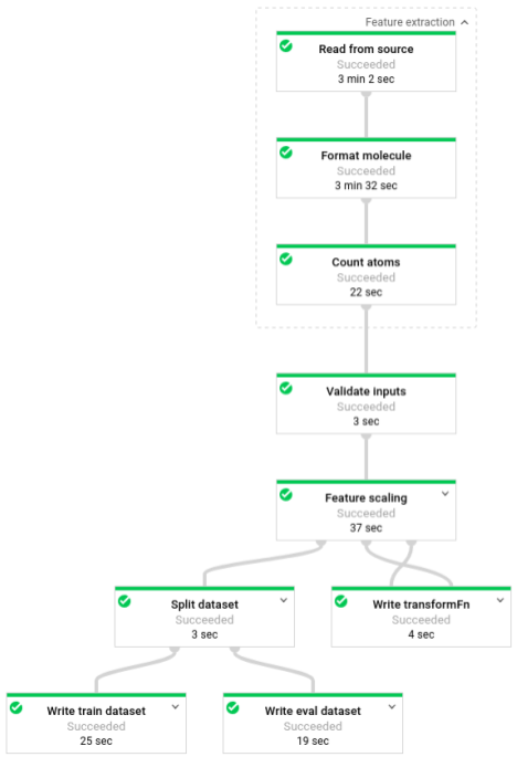
该流水线运行后,您可以在 Dataflow 监控界面中查看流水线的进度:
第 3 阶段:训练
源代码:trainer/task.py
回想一下,在预处理阶段结束时,代码将数据拆分为两个数据集(训练和评估)。
该示例使用 TensorFlow 来训练机器学习模型。分子代码示例中的 trainer/task.py 文件包含用于训练模型的代码。trainer/task.py 的主函数会加载在预处理阶段中处理的数据。
Estimator 会使用训练数据集来训练模型,然后使用评估数据集来验证模型是否能在提供了特定分子属性的情况下准确预测分子能量。
详细了解训练机器学习模型。
训练模型
在本地训练模型:
python trainer/task.py

# To get the path of the trained model
EXPORT_DIR=/tmp/cloudml-samples/molecules/model/export/final
MODEL_DIR=$(ls -d -1 $EXPORT_DIR/* | sort -r | head -n 1)
或者,在 AI Platform 上训练模型:
- 首先,选择一个受支持的区域来运行训练作业
gcloud config set compute/region $REGION
- 启动训练作业
JOB="cloudml_samples_molecules_$(date +%Y%m%d_%H%M%S)"
BUCKET=gs://<your bucket name>
WORK_DIR=$BUCKET/cloudml-samples/molecules
gcloud ai-platform jobs submit training $JOB \
  --module-name trainer.task \
  --package-path trainer \
  --staging-bucket $BUCKET \
  --runtime-version 1.13 \
  --stream-logs \
  -- \
  --work-dir $WORK_DIR

# To get the path of the trained model:
EXPORT_DIR=$WORK_DIR/model/export
MODEL_DIR=$(gsutil ls -d $EXPORT_DIR/* | sort -r | head -n 1)
第 4 阶段:预测
源代码:predict.py
在 Estimator 训练模型后,为模型提供输入即可进行预测。在分子代码示例中,predict.py 中的流水线负责进行预测。该流水线可以作为批处理流水线或流处理流水线。
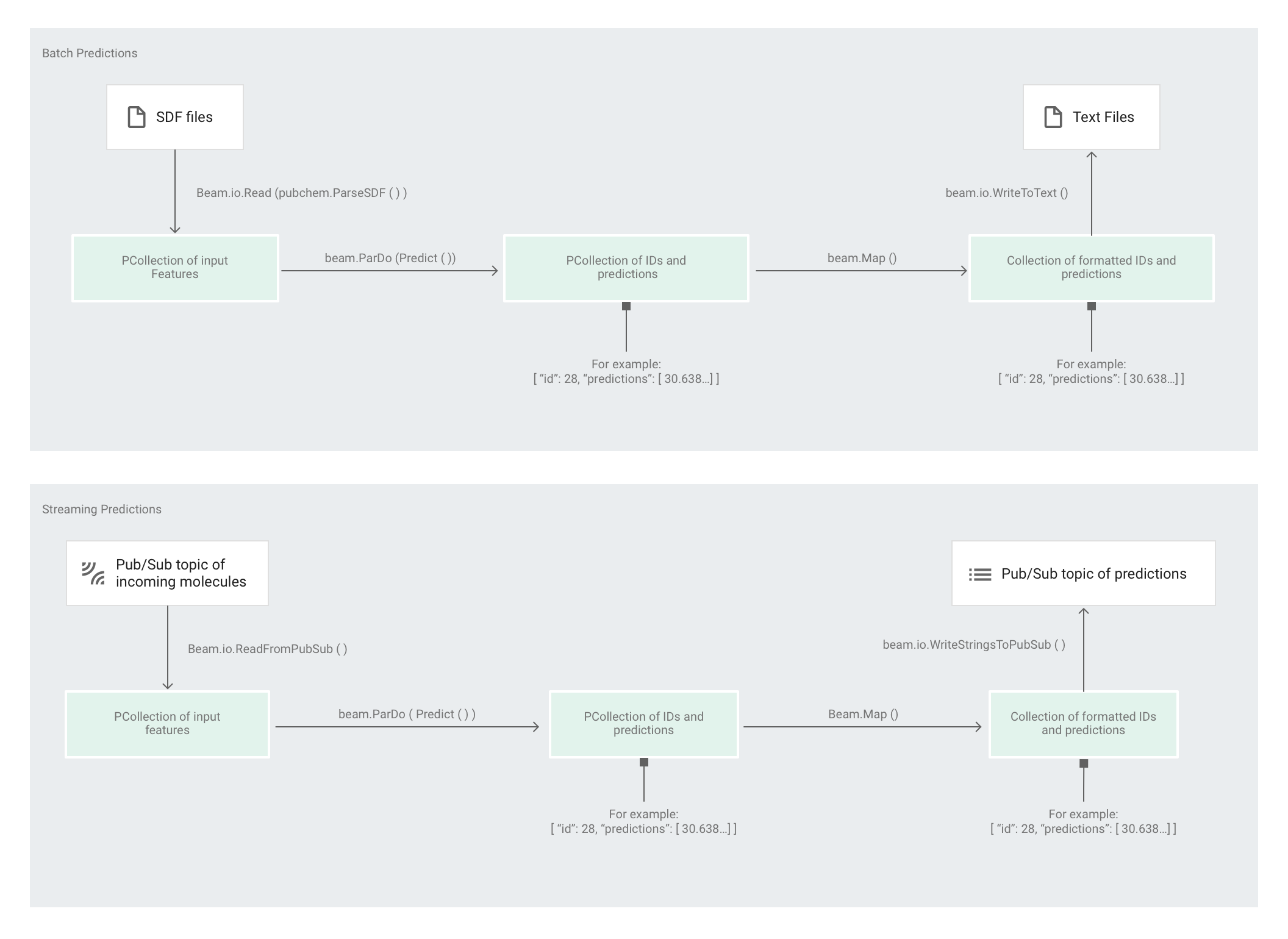
除了来源和接收器交互之外,流水线的代码对于批处理和流处理是相同的。如果流水线以批量模式运行,它将从自定义来源读取输入文件,并将输出预测作为文本文件写入指定的工作目录。如果流水线以流式模式运行,则会在输入分子到达时从某个 Pub/Sub 主题中读取这些输入分子。该流水线会将可供使用的输出预测写入另一个 Pub/Sub 主题。
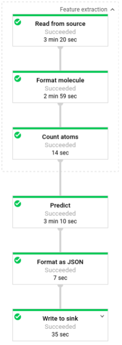
下图显示了预测流水线中的步骤(批处理和流处理)。
在 predict.py 中,代码通过 run 函数定义该流水线:
代码使用以下参数调用 run 函数:
首先,代码会将 pubchem.SimpleFeatureExtraction(source) 转换作为 feature_extraction 转换进行传递。此转换(也用于预处理阶段)会应用于流水线:
该转换基于流水线的执行模式(批处理或流处理)从适当的来源读取分子、设置分子的格式并计算每个分子中不同原子的数量。
接下来,beam.ParDo(Predict(…)) 会应用于执行分子能量预测的流水线。Predict(即系统传递的 DoFn)会使用指定的输入特征(原子计数)字典来预测分子能量。
接着要应用于该流水线的转换是 beam.Map(lambda result: json.dumps(result)),这个转换会获取预测结果字典并将其序列化为 JSON 字符串。
最后,输出会写入接收器(对于批量模式,输出以文本文件形式写入工作目录;对于流式模式,输出以消息形式发布到 Pub/Sub 主题)。
批量预测
批量预测针对吞吐量(而非延迟时间)进行了优化。如果您需要进行许多预测,而且可以等到所有预测完成后再获取结果,则批量预测最适合。
以批量模式运行预测流水线
在本地运行批量预测流水线:
# For simplicity, we'll use the same files we used for training
python predict.py \
  --model-dir $MODEL_DIR \
  batch \
  --inputs-dir /tmp/cloudml-samples/molecules/data \
  --outputs-dir /tmp/cloudml-samples/molecules/predictions
或者,在 Dataflow 上运行批量预测流水线:
# For simplicity, we'll use the same files we used for training
PROJECT=$(gcloud config get-value project)
WORK_DIR=gs://<your bucket name>/cloudml-samples/molecules
python predict.py \
  --work-dir $WORK_DIR \
  --model-dir $MODEL_DIR \
  batch \
  --project $PROJECT \
  --runner DataflowRunner \
  --temp_location $WORK_DIR/beam-temp \
  --setup_file ./setup.py \
  --inputs-dir $WORK_DIR/data \
  --outputs-dir $WORK_DIR/predictions
该流水线运行后,您可以在 Dataflow 监控界面中查看流水线的进度:
流式预测
流式预测针对延迟时间而非吞吐量进行了优化。如果您是零星地进行几次预测,但希望尽快获取结果,则流式预测最适合。
预测服务(流式预测流水线)会从一个 Pub/Sub 主题接收输入分子,并将输出(预测结果)发布到另一个 Pub/Sub 主题。
创建输入 Pub/Sub 主题:
gcloud pubsub topics create molecules-inputs
创建输出 Pub/Sub 主题:
gcloud pubsub topics create molecules-predictions
在本地运行流式预测流水线:
# Run on terminal 1
PROJECT=$(gcloud config get-value project)
python predict.py \
  --model-dir $MODEL_DIR \
  stream \
  --project $PROJECT
  --inputs-topic molecules-inputs \
  --outputs-topic molecules-predictions
或者,在 Dataflow 上运行流式预测流水线:
# Run on terminal 1
PROJECT=$(gcloud config get-value project)
WORK_DIR=gs://<your bucket name>/cloudml-samples/molecules
python predict.py \
  --work-dir $WORK_DIR \
  --model-dir $MODEL_DIR \
  stream \
  --project $PROJECT
  --runner DataflowRunner \
  --temp_location $WORK_DIR/beam-temp \
  --setup_file ./setup.py \
  --inputs-topic molecules-inputs \
  --outputs-topic molecules-predictions
在运行预测服务(流式预测流水线)后,您需要运行发布者服务来将分子发送到预测服务,并运行订阅者服务来侦听预测结果。本分子代码示例提供了发布者 (publisher.py) 和订阅者 (subscriber.py) 服务。
发布者服务会解析目录中的 SDF 文件,并将其发布到输入主题。订阅者服务会侦听预测结果并记录它们。为简单起见,此示例使用与训练阶段相同的 SDF 文件。
运行订阅者服务:
# Run on terminal 2
python subscriber.py \
  --project $PROJECT \
  --topic molecules-predictions
运行发布者服务:
# Run on terminal 3
python publisher.py \
  --project $PROJECT \
  --topic molecules-inputs \
  --inputs-dir $WORK_DIR/data
在发布者服务开始解析和发布分子之后,您将开始看到来自订阅者服务的预测。
清理
在完成流处理预测流水线的运行后,停止您的流水线以防止产生费用。
后续步骤
- 请参阅 Apache Beam 文档
- 阅读 TensorFlow 文档:
- 尝试使用 Apache Beam 和
tf.Transform的其他代码示例。 - 使用 Global Fishing Watch 示例训练机器学习模型以进行时间序列分类。