Continuous model evaluation with BigQuery ML, Stored Procedures, and Cloud Scheduler
Polong Lin
Developer Advocate
Sara Robinson
Staff Developer Relations Engineer
Continuous evaluation—the process of ensuring a production machine learning model is still performing well on new data—is an essential part in any ML workflow. Performing continuous evaluation can help you catch model drift, a phenomenon that occurs when the data used to train your model no longer reflects the current environment.
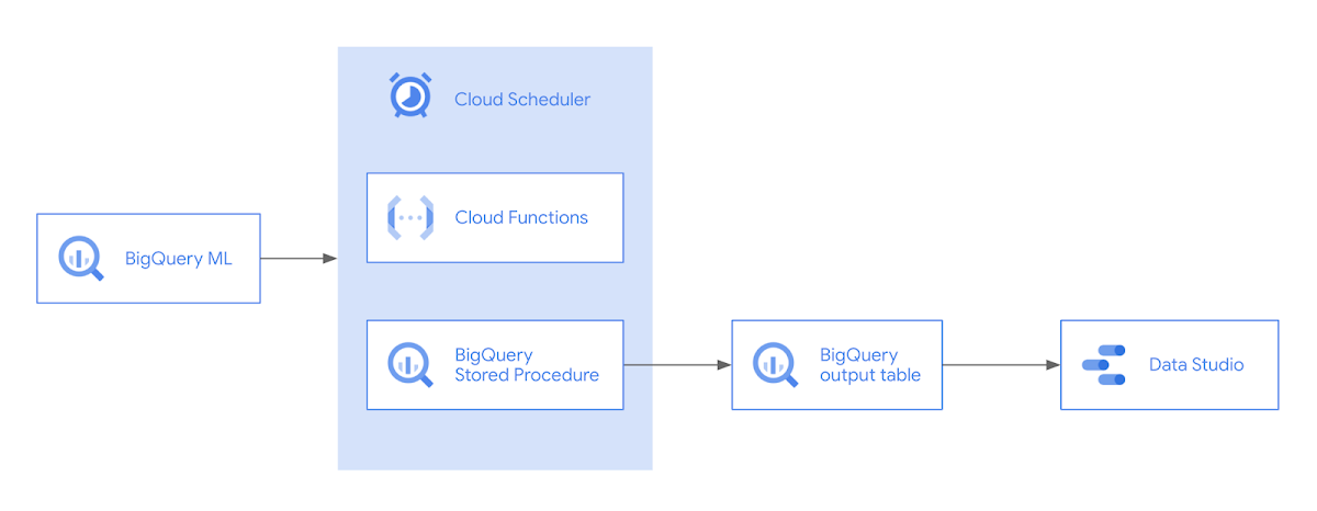
For example, with a model classifying news articles, new vocabulary may emerge that were not included in the original training data. In a tabular model predicting flight delays, airlines may update their routes, leading to lower model accuracy if the model isn’t retrained on new data. Continuous evaluation helps you understand when to retrain your model to ensure performance remains above a predefined threshold. In this post, we’ll show you how to implement continuous evaluation using BigQuery ML, Cloud Scheduler, and Cloud Functions. A preview of what we’ll build is shown in the architecture diagram below.
To demonstrate continuous evaluation, we’ll be using a flight dataset to build a regression model predicting how much a flight will be delayed.
Creating a model with BigQuery ML
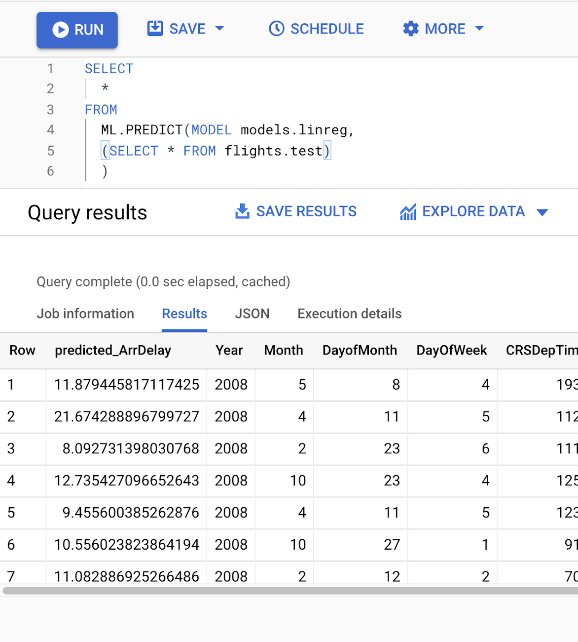
In order to implement continuous evaluation, we’ll first need a model deployed in a production environment. The concepts we’ll discuss can work with any environment you’ve used to deploy your model. Here we’ll use BigQuery Machine Learning (BQML) to build the model. BQML lets you train and deploy models on custom data stored in BigQuery using familiar SQL. We can create our model with the following query:Running this will train our model and create the model resource within the BigQuery dataset we specified in the CREATE MODEL query. Within the model resource, we can also see training and evaluation metrics. When training completes, the model is automatically available to use for predictions via a ML.PREDICT query:
With a deployed model, we’re ready to start continuous evaluation. The first step is determining how often we’ll evaluate the model, which will largely depend on the prediction task. We could run evaluation on a time interval (i.e. once a month), or whenever we receive a certain number of new prediction requests. In this example, we’ll gather evaluation metrics on our model on a daily basis.
Another important consideration for implementing continuous evaluation is understanding when you’ll have ground truth labels available for new data. In our flights example, whenever a new flight lands we’ll know how delayed or early it was. This could be more complex in other scenarios. For example, if we were building a model to predict whether someone will buy a product they add to their shopping cart, we’d need to determine how long we’d wait once an item was added (minutes? hours? days?) before marking it as unpurchased.
Evaluating data with ML.EVALUATE
We can monitor how well our ML model(s) performs over time on new data, by evaluating our models regularly and inserting them into a table on BigQuery.
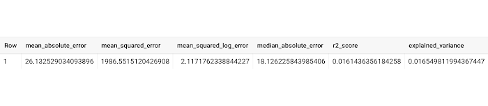
Here's the normal output you would get from using ML.EVALUATE:
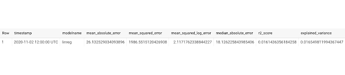
In addition to these metrics, we will also want to store some metadata, such as the name of the model we evaluated and the timestamp of the model evaluation.
But as you can see below, the following code can quickly become difficult to maintain, as every time you execute the query, you would need to replace MY_MODEL_NAME twice (on lines 3 and 6), with the name of the model you created (e.g., "linreg").
Creating a Stored Procedure to evaluate incoming data
You can use a Stored Procedure, which allows you to save your SQL queries and run them by passing in custom arguments, like a string for the model name.
CALL modelevaluation.evaluate("linreg");
Doesn't this look cleaner already?
To create the stored procedure, you can execute the following code, which you can then call using the CALL code shown above. Notice how it takes in an input string, MODELNAME, which then gets used in the model evaluation query.
Another added benefit of stored procedures is that it's much easier to share the query to CALL a stored procedure with others -- which abstracts away from the raw SQL -- rather than share the full SQL query.
Using the Stored Procedure to insert evaluation metrics into a table
Using the stored procedure below, in a single step, we can now evaluate the model and insert it to a table,modelevaluation.metrics, which we will first need to create. This table needs to follow the same schema as in the stored procedure. Perhaps the easiest way is to use LIMIT 0, which is a cost-free query returning zero rows, while maintaining the schema.With the table created, now every time you run the stored procedure on your model "linreg", it will evaluate the model and insert them as a new row into the table:
CALL modelevaluation.evaluate_and_insert("linreg");
Continuous evaluation with Cloud Functions and Cloud Scheduler
To run the stored procedure on a recurring basis, you can create a Cloud Function with the code you want to run, and trigger the Cloud Function with a cron job scheduler like Cloud Scheduler.
Navigating to the Cloud Functions page on Google Cloud Platform, create a new Cloud Function that uses a HTTP trigger type:
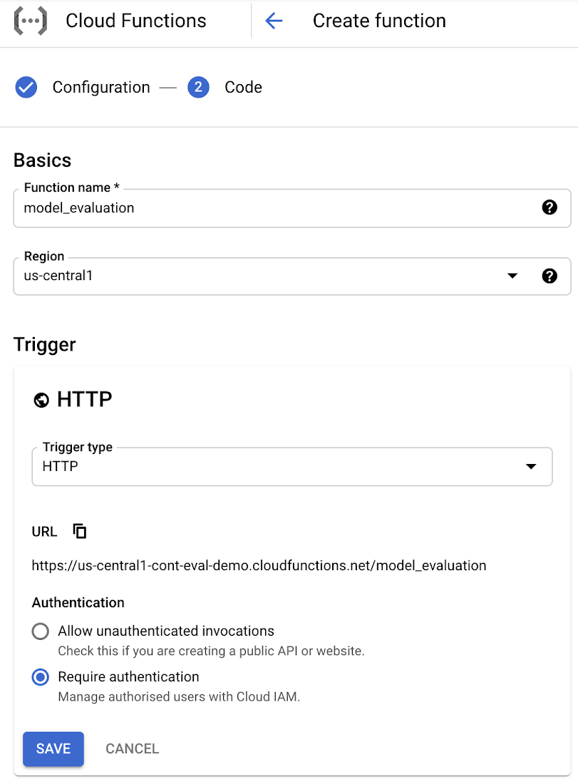
Note the URL, which will be the trigger URL for this Cloud Function. It should look something like:
https://<region>-<projectid>.cloudfunctions.net/<functionname>
Clicking "Next" on your Cloud Functions gets you to the editor, where you can paste the following code, while setting the Runtime to "Python" and changing the "Entry point" to "updated_table_metrics":
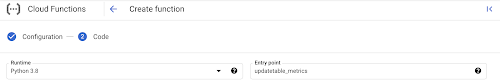
Under main.py, you can use the following code:
Under requirements.txt, you can paste the following code for the required packages:
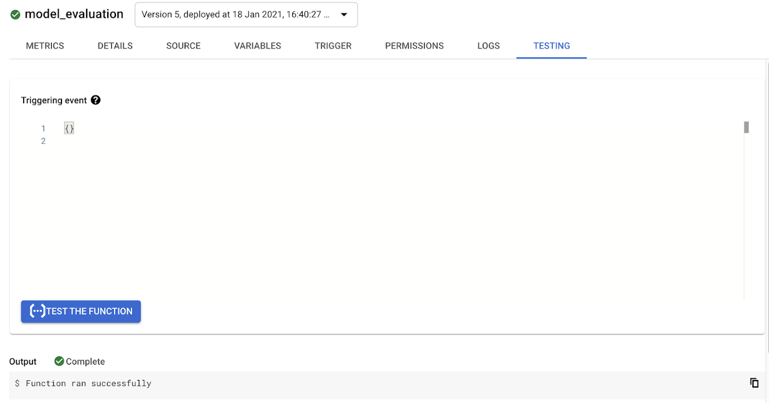
You can then deploy the function, and even test your Cloud Function by clicking on "Test the function" just to make sure it returns a successful response:
Next, to trigger the Cloud Function on a regular basis, we will create a new Cloud Scheduler job on Google Cloud Platform.
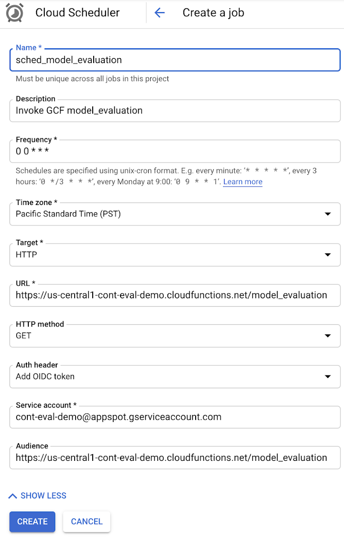
By default, Cloud Functions with HTTP triggers will require authentication, as you probably don't want anyone to be able to trigger your Cloud Functions. This means you will need to include a service account to your Scheduler job that has IAM permissions for:
- Cloud Functions Invoker
- Cloud Scheduler Service Agent
Once the job is created, you can try to run the job by clicking "Run now".
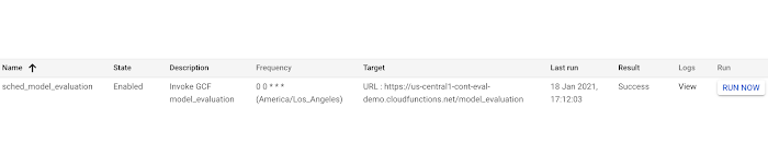
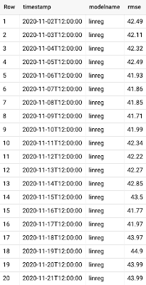
Now you can check your BigQuery table and see if it's been updated! Across multiple days or weeks, you should start to see the table populate, like below:
Visualizing our model metrics
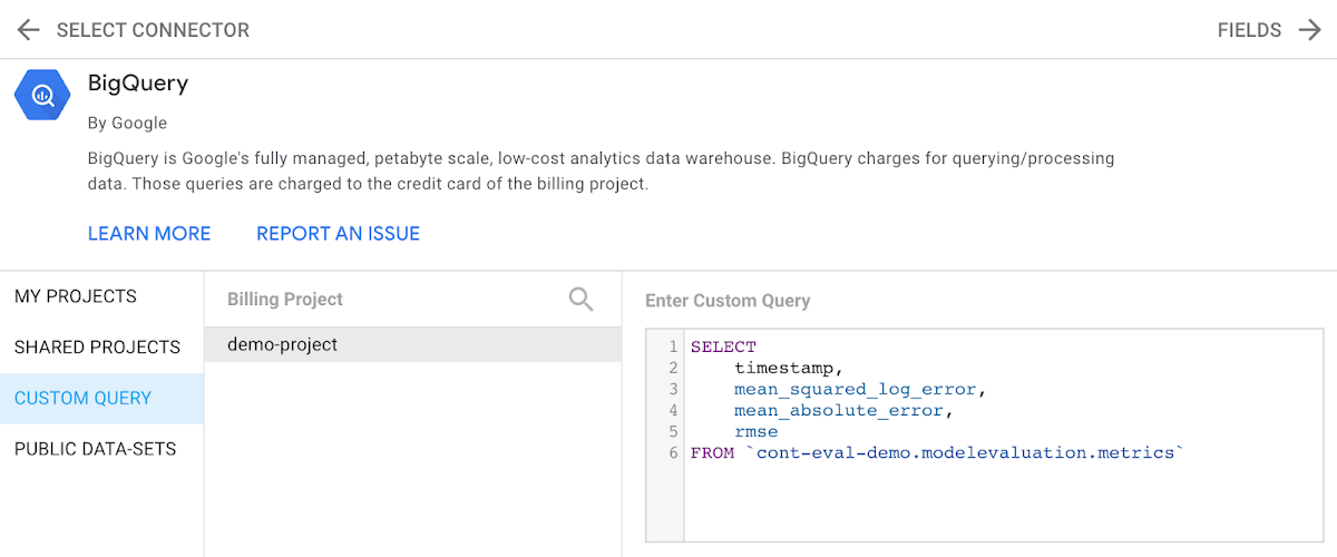
If we’re regularly running our stored procedure on new data, analyzing the results of our aggregate query above could get unwieldy. In that case, it would be helpful to visualize our model’s performance over time. To do that we’ll use Data Studio. Data Studio lets us create custom data visualizations, and supports a variety of different data sources, including BigQuery. To start visualizing data from our BigQuery metrics table, we’ll select BigQuery as a data source, choose the correct project, and then write a query capturing the data we’d like to plot:
For our first chart, we’ll create a time series to evaluate changes to RMSE. We can do this by selecting "timestamp" as our dimension and "rmse" as our metric:
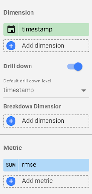
If we wanted more than one metric in our chart, we can add as many as we’d like in the Metric section.
With our metrics selected, we can switch from Edit to View mode to see our time series and share the report with others on our team. In View mode, the chart is interactive so we can see the rmse for any day in the time series by hovering over it:
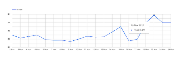
We can also download the data from our chart as a csv or export it to a sheet. From this view, it’s easy to see that our model’s error increased quite a bit on November 19th.
What’s next?
Now that we’ve set up a system for continuous evaluation, we’ll need a way to get alerts when our error goes above a certain threshold. We also need a plan for acting on these alerts, which typically involves retraining and evaluating our model on new data. Ideally, once we have this in place we can build a pipeline to automate the process of continuous evaluation, model retraining, and new model deployment. We’ll cover these topics in future posts - stay tuned!
If you’d like to learn more about any of the topics covered in this post, check out these resources:
Let us know what you thought of this post, and if you have topics you’d like to see covered in the future! You can find us on Twitter at @polonglin and @SRobTweets.