BigQuery Admin reference guide: Storage internals

Leigha Jarett
Developer Advocate, Looker at Google Cloud
So far on the BigQuery Admin Reference Guide series, we’ve talked about the different logical resources available inside of BigQuery. Now, we’re going to begin talking about BigQuery’s architecture. In this post we’re diving into how BigQuery stores your data in native storage, and what levers you can pull to optimize how your data is stored.
Columnar storage format
BigQuery offers fully managed storage, meaning you don’t have to provision servers. Sizing is done automatically and you only pay for what you use. Because BigQuery was designed for large scale data analytics data is stored in columnar format.
Traditional relational databases, like Postgres and MySQL, store data row-by-row in record-oriented storage. This makes them great for transactional updates and OLTP (Online Transaction Processing) use cases because they only need to open up a single row to read or write data. However, if you want to perform an aggregation like a sum of an entire column, you would need to read the entire table into memory.
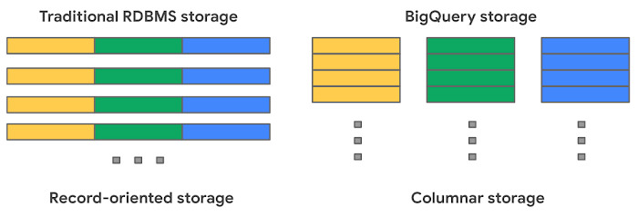
BigQuery uses columnar storage where each column is stored in a separate file block. This makes BigQuery an ideal solution for OLAP (Online Analytical Processing) use cases. When you want to perform aggregations you only need to read the column that you are aggregating over.
Optimized storage format
Internally, BigQuery stores data in a proprietary columnar format called Capacitor. We know Capacitor is a column-oriented format as discussed above. This means that the values of each field, or column, are stored separately so the overhead of reading the file is proportional to the number of fields you actually read. This doesn’t necessarily mean that each column is in its own file, it just means that each column is stored in a file block, which is actually compressed independently for increased optimization.
What’s really cool is that Capacitor builds an approximation model that takes in relevant factors like the type of data (e.g. a really long string vs. an integer) and usage of the data (e.g. some columns are more likely to be used as filters in WHERE clauses) in order to reshuffle rows and encode columns. While every column is being encoded, BigQuery also collects various statistics about the data — which are persisted and used later during query execution.
If you want to learn more about Capacitor, check out this blog post from Google’s own Chief BigQuery Officer.
Encryption and managed durability
Now that we understand how the data is saved in specific files, we can talk about where these files actually live. BigQuery’s persistence layer is provided by Google’s distributed file system, Colossus, where data is automatically compressed, encrypted, replicated, and distributed.
There are many levels of defense against unauthorized access in Google Cloud Platform, one of them being that 100% of data is encrypted at rest. Plus, if you want to control encryption yourself, you can use customer-managed encryption keys.
Colossus also ensures durability by using something called erasure encoding - which breaks data into fragments and saves redundant pieces across a set of different disks. However, to ensure the data is both durable and available, the data is also replicated to another availability zone within the same region that was designated when you created your dataset.
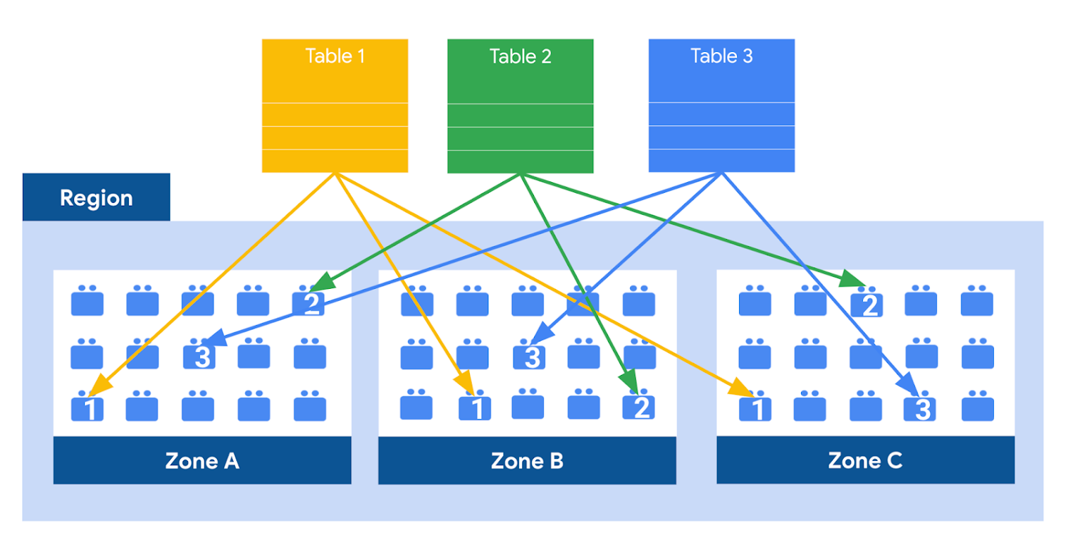
This means data is saved in a different building that has a different power system and network. The chances of multiple availability zones going offline at once is very small. But if you use “Multi-Region” locations - like the US or EU - BigQuery stores another copy of the data in an off-region replica. That way, the data is recoverable in the event of a major disaster.
This is all accomplished without impacting the compute resources available for your queries. Plus encoding, encryption and replication are included in the price of BigQuery storage - no hidden costs!
Optimizing storage for query performance
BigQuery has a built-in storage optimizer that helps arrange data into the optimal shape for querying, by periodically rewriting files. Files may be written first in a format that is fast to write but later BigQuery will format them in a way that is fast to query. Aside from the optimization happening behind the scenes, there are also a few things you can do to further enhance storage.
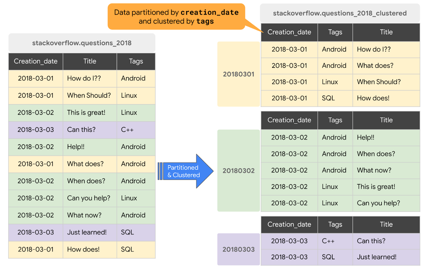
Partitioning
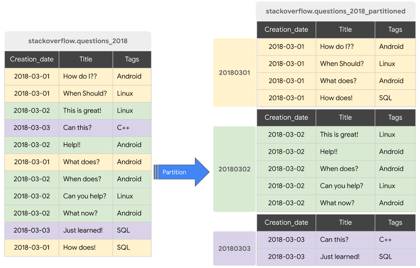
A partitioned table is a special table that is divided into segments, called partitions. BigQuery leverages partitioning to minimize the amount of data that workers read from disk. Queries that contain filters on the partitioning column can dramatically reduce the overall data scanned, which can yield improved performance and reduced query cost for on-demand queries. New data written to a partitioned table is automatically delivered to the appropriate partition.
BigQuery supports the following ways to create partitioned tables:
- Ingestion time partitioned tables: daily partitions reflecting the time the data was ingested into BigQuery. This option is useful if you’ll be filtering data based on when new data was added. For example, the new Google Trends Dataset is refreshed each day, you might only be interested in the latest trends.
- Time-unit column partitioned tables: BigQuery routes data to the appropriate partition based on date value in the partitioning column. You can create partitions with granularity starting from hourly partitioning. This option is useful if you’ll be filtering data based on the date value in the table, for example looking at the most recent transactions by including a WHERE clause for transaction_created_date
- INTEGER range partitioned tables: Partitioned based on an integer column that can be bucketed. This option is useful if you’ll be filtering data based on an integer column in the table, for example focusing on specific customers using customer_id. You can bucket the integer values to create appropriately sized partitions, like having all customers with IDs from 0-100 in the same partition.
Partitioning is a great way to optimize query performance, especially for large tables that are often filtered down during analytics. When deciding on the appropriate partition key, make sure to consider how everyone in your organization is leveraging the table. For large tables that could cause some expensive queries, you might want to require partitions to be used.
Partitions are designed for places where there is a large amount of data and a low number of distinct values. A good rule of thumb is making sure partitions are greater than 1 GB. If you over partition your tables, you’ll create a lot of metadata - which means that reading in lots of partitions may actually slow down your query.
Clustering
When a table is clustered in BigQuery, the data is automatically sorted based on the contents of one or more columns (up to 4, that you specify). Usually high cardinality and non-temporal columns are preferred for clustering, as opposed to partitioning which is better for fields with lower cardinality. You’re not limited to choosing just one, you can have a single table that is both partitioned and clustered!
The order of clustered columns determines the sort order of the data. When new data is added to a table or a specific partition, BigQuery performs free, automatic re-clustering in the background. Specifically, clustering can improve the performance for queries:
- Containing where clauses with a clustered column: BigQuery uses the sorted blocks to eliminate scans of unnecessary data. The order of the filters in the where clause matters, so use filters that leverage clustering first
- That aggregate data based on values in a clustered column: performance is improved because the sorted blocks collocate rows with similar values
- With joins where the join key is used to cluster the table: less data is scanned, for some queries this offers a performance boost over partitioning!
Looking for some more information and example queries? Check out this blog post!
Denormalizing
If you come from a traditional database background, you’re probably used to creating normalized schemas - where you optimize your structure so that data is not repeated. This is important for OLTP workloads (as we discussed earlier) because you’re often making updates to the data. If your customer’s address is stored every place they have made a purchase, then it might be cumbersome to update their address if it changes.
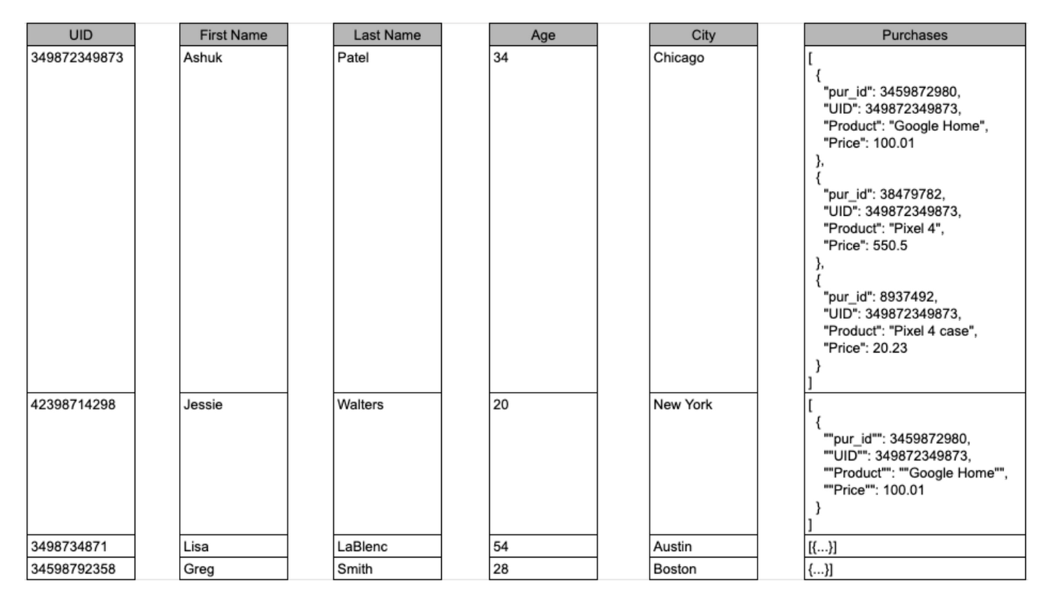
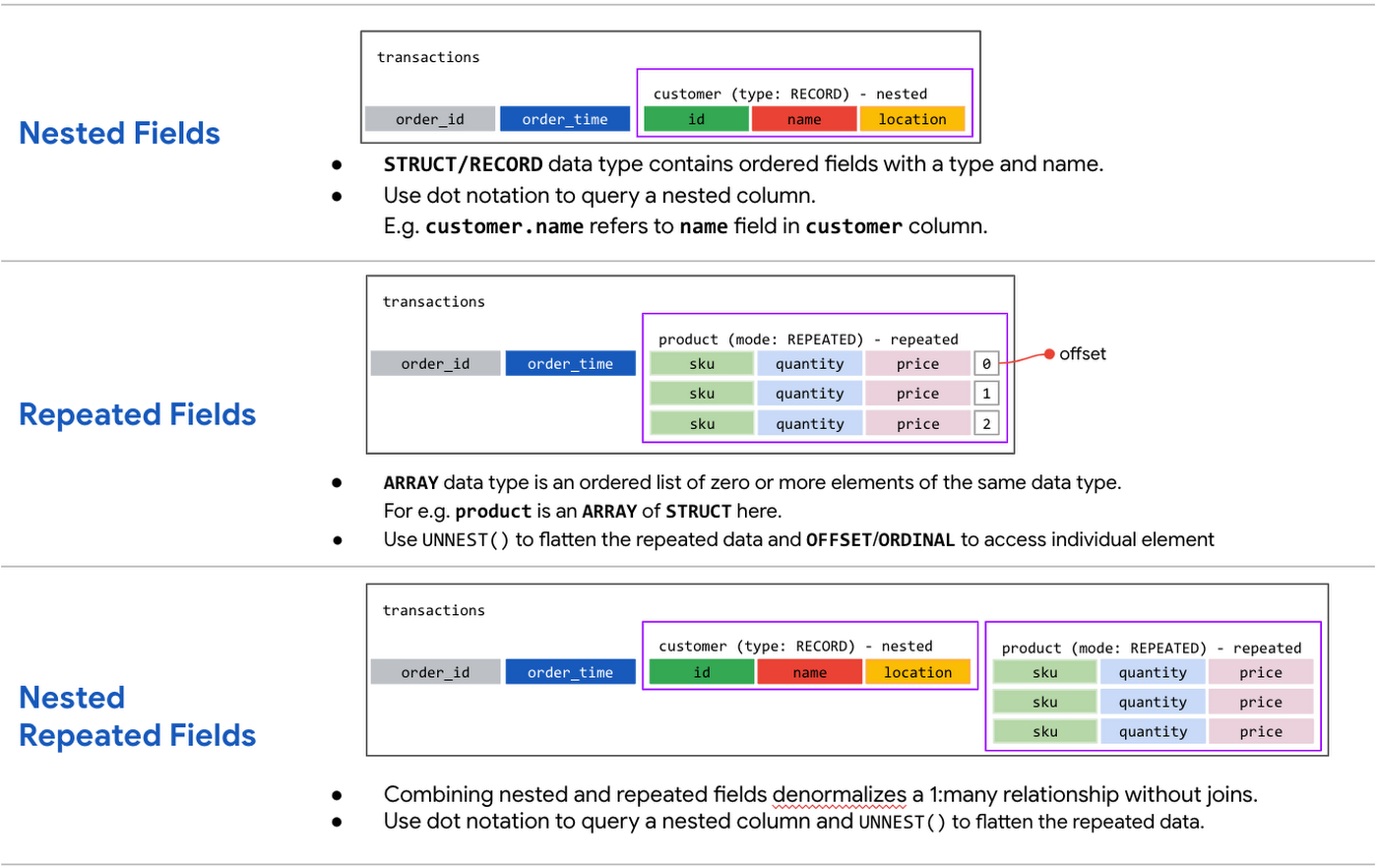
However, when performing analytical operations on normalized schemas, usually multiple tables need to be joined together. If we instead denormalize our data, so that information (like the customer address) is repeated and stored in the same table, then we can eliminate the need to have a JOIN in our query. For BigQuery specifically, we can also take advantage of support for nested and repeated structures. Expressing records using STRUCTs and ARRAYs can not only provide a more natural representation of the underlying data, but in some cases it can also eliminate the need to use a GROUP BY statement. For example, using ARRAY_LENGTH instead of COUNT.
Keep in mind that denormalization has some disadvantages. First off, they aren't storage-optimal. Although, many times the low cost of BigQuery storage addresses this concern. Second, maintaining data integrity can require increased machine time and sometimes human time for testing and verification. We recommend that you prioritize partitioning and clustering before denormalization, and then focus on data that rarely requires updates.
Optimizing for storage costs
When it comes to optimizing storage costs in BigQuery, you may want to focus on removing unneeded tables and partitions. You can configure the default table expiration for your datasets, configure the expiration time for your tables, and configure the partition expiration for partitioned tables. This can be especially useful if you’re creating materialized views or tables for ad-hoc workflows, or if you only need access to the most recent data.
Additionally, you can take advantage of BigQuery’s long term storage. If you have a table that is not used for 90 consecutive days, the price of storage for that table automatically drops by 50 percent to $0.01 per GB, per month. This is the same cost as Cloud Storage Nearline, so it might make sense to keep older, unused data in BigQuery as opposed to exporting it to Cloud Storage.
Thanks for tuning in this week! Next week, we’re talking about query processing - a precursor to some query optimization techniques that will help you troubleshoot and cut costs. Be sure to stay up-to-date on this series by following me on LinkedIn and Twitter!