Getting started with time-series trend predictions using GCP

Today’s financial world is complex, and the old technology used for constructing financial data pipelines isn’t keeping up. With multiple financial exchanges operating around the world and global user demand, these data pipelines have to be fast, reliable and scalable.

Currently, using an econometric approach—applying models to financial data to forecast future trends—doesn’t work for real-time financial predictions. And data that’s old, inaccurate or from a single source doesn’t translate into dependable data for financial institutions to use. But building pipelines with Google Cloud Platform (GCP) can help solve some of these key challenges. In this post, we’ll describe how to build a pipeline to predict financial trends in microseconds. We’ll walk through how to set up and configure a pipeline for ingesting real-time, time-series data from various financial exchanges and how to design a suitable data model, which facilitates querying and graphing at scale.

You’ll find a tutorial below on setting up and deploying the proposed architecture using GCP, particularly these products:

• Cloud Dataflow for a scalable data ingestion system that can handle late data

• Cloud Bigtable, our scalable, low-latency time series database that’s reached 40 million transactions per second on 3,500 nodes. Bonus: A scalable ML pipeline using TensorFlow eXtended, while not part of this tutorial, is a logical next step.

The tutorial will explain how to establish a connection to multiple exchanges, subscribe to their trade feeds, and extract and transform these trades into a flexible format to be stored in Cloud Bigtable and be available to be graphed and analyzed.

This will also set the foundation for ML online learning predictions at scale. You’ll see how to graph the trades, volume, and time delta from trade execution until it reaches our system (an indicator of how close to real time we can get the data). You can find more details on GitHub too.

Before you get started, note that this tutorial uses billable components of GCP, including Cloud Dataflow, Compute Engine, Cloud Storage and Cloud Bigtable. Use the Pricing Calculator to generate a cost estimate based on your projected usage. However, you can try the tutorial for one hour at no charge in this Qwiklab tutorial environment.

Getting started building a financial data pipeline

For this tutorial, we’ll use cryptocurrency real-time trade streams, since they are free and available 24/7 with minimum latency. We’ll use this framework that has all the data exchange streams definitions in one place, since every exchange has a different API to access data streams.

Here’s a look at the real-time, multi-exchange observer that this tutorial will produce:

First, we need to capture as much real-time trading data as possible for analysis. However, the large amount of currency and exchange data available requires a scalable system that can ingest and store such volume while keeping latency low. If the system can’t keep up, it won’t stay in sync with the exchange data stream. Here’s what the overall architecture looks like:

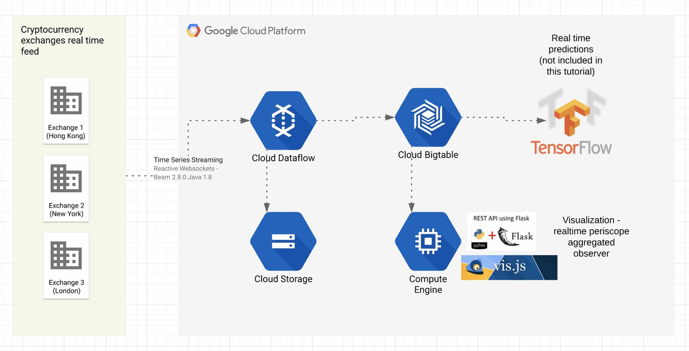
The usual requirement for trading systems is low-latency data ingestion. To this, we add the need for near real-time data storage and querying at scale.

How the architecture works
For this tutorial, the source code is written in Java 8, Python 3, and JavaScript, and we use Maven and PIP for dependency/build management.

There are five main framework units for this code:

1. We’ll use  XChange-stream framework to ingest real-time trading data with low latency from globally scattered data sources and exchanges, with the possibility to adopt data ingest worker pipeline location, and easily add more trading pairs and exchanges. This Java library provides a simple and consistent streaming API for interacting with cryptocurrency exchanges via WebSocket protocol. You can subscribe for live updates via reactive streams of RxJava library. This helps connect and configure some exchanges, including BitFinex, Poloniex, BitStamp, OKCoin, Gemini, HitBTC and Binance.

2. For parallel processing, we’ll use  Apache Beam for an unbounded streaming source code that works with multiple runners and can manage basic watermarking, checkpointing and record ID for data ingestion. Apache Beam is an open-source unified programming model to define and execute data processing pipelines, including ETL and batch and stream (continuous) processing. It supports Apache Apex, Apache Flink, Apache Gearpump, Apache Samza, Apache Spark, and Cloud Dataflow.

3. To achieve strong consistency, linear scalability, and super low latency for querying the trading data, we’ll use  Cloud Bigtable with Beam using the HBase API as the connector and writer to Cloud Bigtable. See how to create a row key and a mutation function prior to writing to Cloud Bigtable.

4. For a real-time API endpoint , we’ll use a  Flask web server at port:5000 plus a Cloud Bigtable client to query Cloud Bigtable and serve as an API endpoint. We’ll also use a JavaScript visualization  with a Vis.JS Flask template to query the real-time API endpoint every 500ms. The Flask web server will run in the GCP VM instance.

5. For easy and automated setup with project template for orchestration, we’ll use Terraform. Here’s an example of dynamic variable insertion from the Terraform template into the GCP compute instance.

Define the pipeline
For every exchange and trading pair, create a different pipeline instance. This consists of three steps:

1. UnboundedStreamingSource that contains ‘UnboundedStreamingSourceReader’

2. Cloud Bigtable pre-writing mutation and key definition

Cloud Bigtable write step

Make the Cloud Bigtable row key design decisions
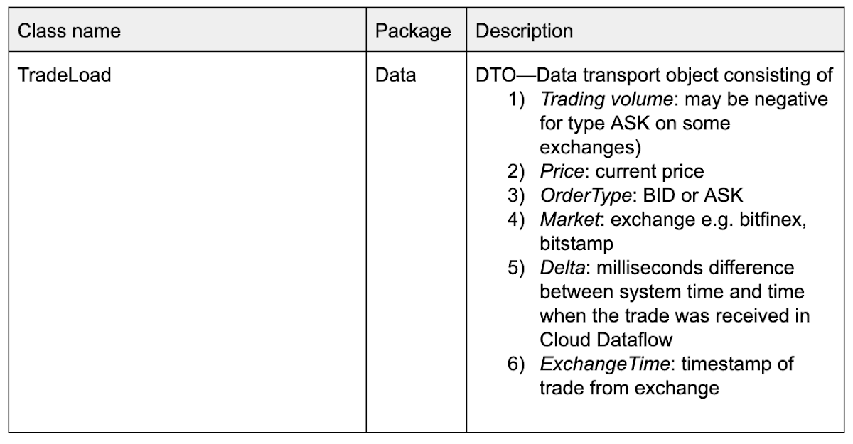
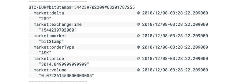
In this tutorial, our data transport object looks like this:

We formulated the row key structure like this: TradingCurrency#Exchange#SystemTimestampEpoch#SystemNanosTime.

So a row key might look like this: BTC/USD#Bitfinex#1546547940918#63187358085 with these definitions:

BTC/USD: trading Pair

Bitfinex :  exchange

1546547940918:  Epoch timestamp

63187358085:  System nanotime

We added nanotime at our key end to help avoid multiple versions per row for different trades. Two DoFn mutations might execute in the same Epoch millisecond time if there is a streaming sequence of TradeLoad DTOs, so adding nanotime at the end will split the millisecond to an additional one million.

We also recommend hashing the volume-to-price ratio and attaching the hash at the end of the row key. Row cells will contain an exact schema replica of the exchange TradeLoad DTO (see the table above). This choice helps move from the specific (trading pair to exchange) to the general (timestamp  to  nanotime), avoiding hotspots when you query the data.

Set up the environment
If you are familiar with Terraform, it can save you a lot of time setting up the environment using Terraform instructions. Otherwise, keep reading.

First, you should have a Google Cloud project associated with a billing account (if not, check out the getting started section). Log into the console, and activate a cloud console session.

Next, create a VM with the following command:

Note that we used the Compute Engine Service Account with Cloud API scope to make it easier to build up the environment.

Wait for the VM to come up and SSH into it.

Next, enable some APIs and create a Cloud Bigtable instance and bucket:

In this scenario, we use a one-column family called “market” to simplify the Cloud Bigtable schema design (more on that here):

Once that’s ready, clone the repository:

Then build the pipeline:

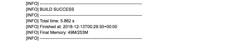
If everything worked, you should see this at the end and can start the pipeline:

Ignore any illegal thread pool exceptions. After a few minutes, you’ll see the incoming trades in the Cloud Bigtable table:

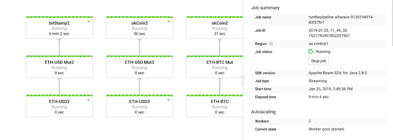
To observe the Cloud Dataflow pipeline, navigate to the Cloud Dataflow console page. Click on the pipeline and you’ll see the job status is “running”:

Add a visualization to your data
To run the Flask front-end server visualization to further explore the data, navigate to the front-end directory inside your VM and build the Python package.

Open firewall port 5000 for visualization:

Link the VM with the firewall rule:

Then, navigate to the front-end directory:

Find your external IP in the Google Cloud console and open it in your browser with port 5000 at the end, like this: http://external-ip:5000/stream

You should be able to see the visualization of aggregated BTC/USD pair on several exchanges (without the predictor part). Use your newfound skills to ingest and analyze financial data quickly!

Clean up the tutorial environment

We recommend cleaning up the project after finishing this tutorial to return to the original state and avoid unnecessary costs.

You can clean up the pipeline by running the following command:

Then empty and delete the bucket:

Delete the Cloud Bigtable instance:

Exit the VM and delete it from the console.

Learn more about Cloud Bigtable schema design for time series data, Correlating thousands of financial time series streams in real time, and check out other Google Cloud tips.

Special thanks to contributions from: Daniel De Leo, Morgante Pell, Yonni Chen and Stefan Nastic.
Google does not endorse trading or other activity from this post and does not represent or warrant to the accuracy of the data.