Take a tour of best practices for Cloud Bigtable performance and cost optimization

To serve your various application workloads, Google Cloud offers a selection of managed database options: Cloud SQL and Cloud Spanner for relational use cases, Firestore and Firebase for document data, Memorystore for in-memory data management, and Cloud Bigtable, a wide-column, NoSQL key-value database. 

Bigtable was designed by Google to store, analyze, and manage petabytes of data while supporting horizontal scalability to millions of requests per second at low latency. Cloud Bigtable offers Google Cloud customers this same database that has been battle tested within Google for over a decade, without the operational overhead of traditional self-managed databases. When considering the total cost of ownership, fully managed cloud databases are often far less expensive to operate than self-managed databases. Nonetheless, as your databases continue to support your growing applications, there are coincident opportunities to optimize cost. 

This blog provides best practices for optimizing a Cloud Bigtable deployment for cost savings. A series of options are presented and the respective tradeoffs to be considered are discussed.

Before you begin

Written for developers, database administrators, and system architects who currently use Cloud Bigtable, or are considering using it, this blog will help you strike the right balance between performance and cost. 

The first installment in this blog series, A primer on Cloud Bigtable cost optimization, reviews the billable components of Cloud Bigtable, discusses the impact various resource changes can have on cost, and introduces the best practices that will be covered in more detail in this article.

Note: This blog does not replace the public Cloud Bigtable documentation, and you should be familiar with that documentation before you read this guide. Further, this article is not intended to go into the details of optimizing a particular workload to support a business goal, but instead provides some general best practices that can be employed to balance cost and performance.

Understand the current database behavior

Before you make any changes, spend some time to observe and document the current behavior of your clusters. 

Use Cloud Bigtable Monitoring to document and understand the existing values and trends for these key metrics:

• Reads/writes per second 

• CPU utilization 

• Request latency

• Read/write throughput

• Disk usage

You will want to look at the metric values at various points throughout the day, as well as the longer-term trends. To start, look at the current and previous weeks to see if the values are constant throughout the day, follow a daily cycle, or follow some other periodic pattern. Assessing longer periods of time can also provide valuable insight, as there may be monthly or seasonal patterns.

Take some time to review your workload requirements, use-cases and access patterns. For instance, are they read-heavy or write-heavy? Or, are they throughput or latency sensitive? Knowledge of these constraints will help you balance performance with costs. 

Define minimum acceptable performance thresholds 

Before making any changes to your Cloud Bigtable cluster, take a moment to acknowledge the potential tradeoffs in this optimization exercise. The goal is to reduce operational costs by reducing your cluster resources, changing your instance configuration, or reducing storage requirements to the minimum resources required to serve your workload according to your performance requirements. Some resource optimization may be possible without any effect on your application performance, but more likely, cost-reducing changes will influence application performance metric values. Knowing the minimum acceptable performance thresholds for your application is important so that you know when you have reached the optimal balance of cost and performance.

First, create a metric budget. Since you will use your application performance requirements to drive the database performance targets, take a moment to quantify the minimum acceptable latency and throughput metric values for each application use case. These values represent the use case metric budget total. For a given use case, you may have numerous backend services which interact with Cloud Bigtable to support your application. Use your knowledge of the respective backend services and their behaviors to allocate to each backend service a fraction of the total budget. It is likely, each use case is supported by more than one backend service, but if Cloud Bigtable is the only backend service, then the entire metric budget can be allocated to Cloud Bigtable. 

Now, compare the measured Cloud Bigtable metrics with the available metric budget. If the budget is greater than the metrics which you observed, there is room to reduce the resources provisioned for Cloud Bigtable without making any other changes. If there is no headroom when you compare the two, you will likely need to make architectural or application logic changes before the provisioned resources can be reduced.

This diagram shows an example of the apportioned metric budget for latency for an Application, which has two use cases. Each of these use cases call backend services, which in turn use additional backend services as well as Cloud Bigtable.

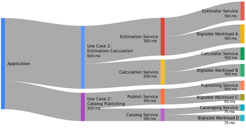
Notice in the examples shown in the illustration above that the budget available for the Cloud Bigtable operations is only a portion of the total service call budget. For instance, the Estimation Service has a total budget of 300ms and the component call to Cloud Bigtable Workload A has been allotted a minimum acceptable performance threshold of 150ms. As long as this database operation finishes in 150ms or less, the budget has not been exhausted. If, when reviewing your actual database metrics, you find that Cloud Bigtable Workload A is completing more quickly than this, then you have some room to maneuver in your budget that may provide an opportunity to reduce your compute costs.

Four methods to balance performance and cost

Now that you have a better understanding of the behavior, and resource requirements for your workload, you can consider the available opportunities for cost optimization. 

Next, we’ll cover four potential and complementary methods to help you:

• Size your cluster optimally

• Optimize your database performance

• Evaluate your data storage usage

• Consider architectural alternatives

Method 1: Size clusters to an optimal cluster node count

Before you consider making any changes to your application or data serving architecture, make certain that you have optimized the number of nodes provisioned for your clusters for your current workloads.

Assess observed metrics for overprovisioning signals

For single clusters, or multi-cluster instances with single-cluster routing, the recommended maximum average CPU utilization is 70% for the cluster and 90% for the hottest node. For an instance composed of multiple clusters with multi-cluster routing, the recommended maximum average CPU utilization is 35% for the cluster and 45% for the hottest node.

Compare the appropriate recommended maximum values for CPU utilization value to the metric trends you observe on your existing cluster(s). If you find a cluster with average utilization significantly lower than the recommended value, the cluster is likely underutilized and could be a good candidate for downsizing. Keep in mind that instance clusters need not have a symmetric node count; you can size each cluster in an instance according to its utilization.

When you compare your observations with the recommended values, take into account the various periodic maximums you observed when assessing the cluster metrics. For example, if your cluster utilizes a peak weekday average of 55% CPU utilization, but also reaches a maximum average of 65% on the weekend, the later metric value should be used to determine the CPU headroom in your cluster.

Manually optimize node count 

To right-size your cluster following this strategy: decrease the number of nodes slowly, and observe any change in behavior during a period of time when the cluster has reached a steady state. A good rule of thumb is to reduce the cluster node count by no more than 5% to 10% every 10 to 20 minutes. This will allow the cluster to smoothly rebalance the splits as the number of serving nodes decreases. 

When planning modifications to your instances, take your application traffic patterns into consideration. For instance, monitoring during off-hours may give false signals when determining the optimal node count. Traffic during the modification period should be representative of a typical application load. For example, downsizing and monitoring during off-hours may give false signals when determining the optimal node count. 

Keep in mind that any changes to your database instance should be complemented by active monitoring of your application behavior. As the node count decreases, you will observe a corresponding increase in average CPU increase. When it reaches the desired level, no additional nodes reduction is needed. If, during this process, the CPU value is higher than your target, you will need to increase the number of nodes in the cluster to serve the load.

Use autoscaling to maintain node count at an optimal level over time

In the case that you observed a regular daily, weekly, or seasonal pattern when assessing the metric trends, you might benefit from metric-based or schedule-based autoscaling. With a well formulated auto-scaling strategy in place, your cluster will expand when additional serving capacity is necessary and contract when need has subsided. On average, you will have a more cost efficient deployment that meets your application performance goals.

Because Cloud Bigtable does not provide a native autoscaling solution just yet, you can use the Cloud Bigtable Admin API to programmatically resize your clusters. We’ve seen customers build their own autoscaler using this API. One such open source solution for Cloud Bigtable autoscaling that has been reused by numerous Google Cloud customers is available on GitHub. 

As you implement your auto-scaling logic, here are some helpful pointers:

• Scale up/down according to a measured strategy. When scaling up, consider cost. Scaling up too quickly will lead to increased costs. When scaling down, scale down gradually for optimal performance. 

• Frequent increases and decreases in cluster node count in a short time period are cost ineffective. Since you are charged each hour for the maximum number of nodes that exist during that hour, granular up and down scaling within an hour will be cost inefficient.

• Autoscaling is only effective for the right workloads. There is a short lag time, on the order of minutes, after adding nodes to your cluster before they can serve traffic effectively. This means that autoscaling is not an ideal solution for addressing short-duration traffic bursts. 

• Choose autoscaling for traffic that follows a periodic pattern. Autoscaling works well for solutions with normal, diurnal traffic patterns like scheduled batch workloads or an application where traffic patterns follow normal business hours. 

• Autoscaling is also effective for bursty workloads. For workloads that anticipate scheduled batch workloads an autoscaling solution with scheduling capability to scale up in anticipation of the batch traffic can work well

Method 2: Optimize database performance to lower cost

If you can reduce the database CPU load by improving the performance of your application or optimizing your data schema, this will, in turn, provide the opportunity to reduce the number of cluster nodes. As discussed, this would then lower your database operational costs.

Apply best practices to rowkey design to avoid hotspots

It's worth repeating: the most frequently experienced performance issues for Cloud Bigtable are related to rowkey design, and of those, the most common performance issues result from data access hotspots. As a reminder, a hotspot occurs when a disproportionate share of database operations interact with data in an adjacent rowkey range. Often, hotspots are caused by rowkey designs consisting of monotonically increasing values such as sequential numeric identifiers or timestamp values. Other causes include frequently updated rows, and access patterns resulting from certain batch jobs.

You can use Key Visualizer to identify hotspots and hotkeys in your Cloud Bigtable clusters. This powerful monitoring tool generates visual reports for each of your tables, showing your usage based on the rowkeys that are accessed. Heatmaps provide a quick method to visually inspect table access to identify common patterns including periodic usage spikes, read or write pressure for specific hotkey ranges, and telltale signs of sequential reads and writes.

If you identify hotspots in your data access patterns, there are a few strategies to consider: 

• Ensure that your rowkey space is well-distributed

• Avoid repeatedly updating the same row with new values; It is far more efficient to create new rows.

• Design batch jobs to access data in a well-distributed pattern

Consolidate datasets with similar schema and contemporaneous access

You may be familiar with database systems where there are benefits in manually partitioning data across multiple tables, or in normalizing relational schema to create more efficient storage structures. However, in Cloud Bigtable, it can often be better to store all your data in one (no pun intended) big table. 

The best practice is to design your tables to consolidate datasets into larger tables in cases where they have similar schema, or they consist of data, in columns or adjacent rows, that are concurrently accessed.

There are a few reasons for this strategy: 

• Cloud Bigtable has a limit of 1,000 tables per instance. 

• A single request to a larger table can be more efficient than concurrent requests to many smaller tables.

• Larger tables can take better advantage of the load-balancing features that provide the high performance of Cloud Bigtable.

Further, since Key Visualizer is only available for tables with at least 30 GB of data, table consolidation might provide additional observability. 

Compartmentalize datasets which are not accessed together

For example, if you have two datasets, and one dataset is accessed less frequently than the other, designing a schema to separate these datasets on disk might be beneficial. This is especially true if the less frequently accessed dataset is much larger than the other, or if the rowkeys of the two datasets are interleaved.

There are several design strategies available to compartmentalize dataset storage.

If atomic row-level updates are not required, and the data is rarely accessed together, two options can be considered:

• Store the data in separate tables. Even if both datasets share the same rowkey space, the datasets can be separated into two separate tables. 

• Keep the data in one table but use separate rowkey prefixes to store related data in contiguous rows, in order to separate the disparate dataset rows from each other. 

If you need atomic updates across datasets which share a rowkey space, you will want to keep those datasets in the same table, but each dataset can be placed in a different column family. This is especially effective if your workload concurrently ingests the disparate datasets with the shared keyspace, but reads those datasets separately.

When a query uses a Cloud Bigtable Filter to ask for columns from just one family, Cloud Bigtable efficiently seeks the next row when it reaches the last of that column family's cells. In contrast, if independently requested column sets are interleaved within a single column family, Cloud Bigtable will not be able to read the desired cells contiguously. Due to the layout of data on disk, this results in a more resource-expensive series of filtering operations to retrieve the requested cells one at a time.

These schema design recommendations have the same result: The two datasets will be more addressable on disk, which makes the frequent accesses to the smaller dataset much more efficient. Further, separating data which you write together but do not read together lets Cloud Bigtable more efficiently seek the relevant blocks of the SSTable and skip past irrelevant blocks. Generally, any schema design changes made to control relative sort order can potentially help improve performance, which in turn could reduce the number of needed compute nodes, and deliver cost savings.

Store many column values in a serialized data structure 

Each cell traversed by a read incurs a small additional overhead, and each cell returned comes with further overhead at each level of the stack. You may realize performance gains, if you store structured data in a single column as a blob rather than spreading it across a row with one value per column.

There are two exceptions to this recommendation.

First, if the blob is large and you frequently only want part of it, splitting up the data can result in higher data throughput. If your queries generally target disjointed subsets of the data, make a column for each respective smaller blob. If there's some overlap, try a tiered system. For example, you might make columns A, B, and C to support queries which just want blob A, sometimes request blobs A and B or blobs B and C, but rarely require all three.

Second, if you want to use Cloud Bigtable filters (see caveats above) on a portion of the data, that section will need to be in its own column.

If this method fits your data and use-case, consider using the protocol buffer (Protobuf) binary format that may reduce storage overhead as well as improve performance. The tradeoff is that additional client side processing will be required to decode the protobuf to extract data values. (Check out the post on the two sides of this tradeoff and potential cost optimization for more detail.) 

Consider use of timestamps as part of the rowkey

If you are keeping multiple versions of your data, consider adding timestamps at the end of your rowkey instead of keeping multiple timestamped cells of a column in a row. 

This changes the disk sort order from (row, column, timestamp) to (row, timestamp, column). In the former case, the cell timestamp is assigned as part of the row mutation, and is a final part of the cell identifier. In the latter case, the data timestamp is explicitly added to the rowkey. This latter rowkey design is much more efficient if you want to retrieve many columns per row but only a single timestamp or limited range of timestamps. 

This approach is complementary to the previous serialized structure recommendation: if you collect multiple timestamped cells for each column, an equivalent serialized data structure design will require the timestamp to be promoted to the rowkey. If you cannot store all columns together in a serialized structure, storing values in individual columns will still provide benefits if you read columns in a manner well-suited to this pattern.

If you frequently add new timestamped data for an entity in order to persist a time series, this design is most advantageous. However, if you only keep a few versions for historical purposes, intrinsic Cloud Bigtable timestamped cells will be preferable, as these timestamps are obtained and applied to the data automatically, and will not have a detrimental performance impact. Keep in mind, if you only have one column, the two sort orders are equivalent.

Consider client filtering logic over complex query filter predicates

The Cloud Bigtable API has a rich, chainable, filtering mechanism which can be very useful when searching a large dataset for a small subset of results. However, if your query is not very selective in the range of rowkeys requested, it is likely more efficient to return all the data as fast as possible and filter in your application. To justify the increased processing cost, only queries with a selective result set should be written with server-side filtering.

Utilize garbage-collection policies to automatically minimize row size

While Cloud Bigtable can support rows with data up to 256MB in size, performance may be impacted if you store data in excess of 100 MB per row. Since large rows negatively affect performance, you will want to prevent unbounded row growth. You could explicitly delete the data by removing unneeded cells, column families or rows, however this process would either have to be performed manually or would require automation, management, and monitoring.

Alternatively, you can set a garbage-collection policy to automatically mark cells for deletion at the next compaction, which typically takes a few days but might take up to a week. You can set policies, by column family, to remove cells that exceed either a fixed number of versions, or an age-based expiration, commonly known as a time to live (TTL). It is also possible to apply one of each policy type and define the mechanism of combined application: either the intersection (both) or the union (either) of the rules.

There are some subtleties on the exact timing of when data is removed from query results that are worth reviewing: explicit deletes, those that are performed by the Cloud Bigtable Data API DeleteFromRow Mutation, are immediately omitted, whereas the specific moment a garbage collected cell is excluded cannot be guaranteed.

Once you have assessed your requirements for data retention, and understand the growth patterns for your various datasets, you can develop a strategy for garbage-collection that will ensure row sizes do not have an adverse effect on performance by exceeding the recommended maximum size.

Method 3: Evaluate data storage for cost saving opportunities

While more likely that Cloud Bigtable nodes account for a large proportion of your monthly spend, you should also evaluate your storage for cost reduction prospects. As separate line items, you are billed for the storage used by Cloud Bigtable's internal representation on disk, and for the compressed storage required to retain any active table backups.

There are several active and passive methods at your disposal to control data storage costs.

Utilize garbage-collection policies to remove data automatically

As discussed above, the use of garbage-collection policies can simplify dataset pruning. In the same way that you might choose to control the size of rows to ensure proper performance, you can also set policies to remove data to control data storage costs. 

Garbage collection allows you to save money by removing data that is no longer required or used. This is especially true if you are using the SSD storage type.

In the case that you want to apply garbage-collection policies to serve both this purpose and the one earlier discussed you can use a policy based on multiple criteria: either a union policy or a nested policy with both an intersection and a union. 

To take an extreme example, imagine you have a column that stores values of approximately 10 MB, so you would need to make sure that no more than ten versions are held to keep the row size below 100 MB. There is business value in keeping these 10 versions for the short term, but in the long term, in order to control the amount of data storage, you only need to keep a few versions. 

In this case you could set such a policy: (maxage=7d and maxversions=2) or maxversions=10. 

This garbage collection policy would removes cells in the column family that meet either of the following conditions:

• Older than the 10 most recent cells

• More than seven days old and older than the two most recent cells

A final note on garbage-collection policies: do take into consideration that you will continue to be charged for storage of expired or obsolete data until compaction occurs (when garbage-collection happens) and the data is physically removed. This process typically will occur within a few days but might require up to a week. 

Choose a cost-aware backup plan 

Database backups are an essential aspect of a backup and recovery strategy. With Cloud Bigtable managed table backups, you can protect your data against operator error and application data corruption scenarios. Cloud Bigtable backups are handled entirely by the Cloud Bigtable service, and you are only charged for storage during the retention period. Since there is no processing cost to create or restore a backup, they are less expensive than external backups that export, and import data using separately provisioned services. 

Table backups are stored with the cluster where the backup was initiated and include, with some minor caveats, all the data that was in the table at backup creation time. When a backup is created, a user-defined expiration date is defined. While this date can be up to 30 days after the backup is created, the retention period should be carefully considered so that you do not keep it longer than necessary. You can establish a retention period according to your requirements for backup redundancy and table backup frequency. The latter should reflect the amount of acceptable data loss: the recovery point objective (RPO) of your backup strategy.

For example, if you have a table with an RPO of one hour, you can configure a schedule to create a new table backup every hour. You could set the backup expiration to the 30 day maximum, however this setting would, depending on the size of the table, incur a significant cost. Depending on your business requirements, this cost might not provide a correlative value. Alternatively, based on your backup retention policy, you could choose to set a much shorter backup expiration period: for example, four hours. In this hypothetical example, you could recover your table within the required RPO of less than one hour, yet at any point in time you would only retain four or five table backups. This is in comparison to 720 backups, if backup expiration was set to 30 days. 

Provision with HDD storage

When a Cloud Bigtable instance is created, you must choose between SSD or HDD storage. SSD nodes are significantly faster with more predictable performance, but come at a premium cost and lower storage capacity per node. Our general recommendation is: choose SSD storage when in doubt. However, an instance with HDD storage can provide significant cost savings for workloads of a suitable use case. 

Signs that your use case may be a good fit for HDD instance storage include:

• Your use case has large storage requirements (greater than 10 TB) especially relative to the anticipated read throughput. For example, a time series database for classes of data, such as archival data, that are infrequently read 

• Your use case data access traffic is largely composed of writes, and predominantly scan reads. HDD storage provides reasonable performance for sequential reads and writes, but only supports a small fraction of the random read rows per second provided by SSD storage.

• Your use case is not latency sensitive. For example, batch workloads that drive internal analytics workflows. 

That being said, this choice must be made judiciously. HDD instances can be more expensive than SSD instances if, due to the differing characteristics of the storage media, your cluster becomes disk I/O bound. In this circumstance, an SSD instance could serve the same amount of traffic with fewer nodes than an HDD instance. Moreover, the instance store type cannot be changed after creation time; to switch between SSD and HDD storage types, you would need to create a new instance and migrate the data. Review the Cloud Bigtable documentation for a more thorough discussion of the tradeoffs between SSD and HDD storage types. 

Method 4: Consider architectural changes to lower database load 

Depending on your workload, you might be able to make some architectural changes to reduce the load on the database, which would allow you to decrease the number of nodes in your cluster. Fewer nodes will result in a lower cluster cost.

Add a capacity cache

Cloud Bigtable is often selected for its low latency in serving read requests. One of the reasons it works great for these types of workloads is that Cloud Bigtable provides a Block Cache that caches SSTables blocks that were read from Colossus, the underlying distributed file system. Nonetheless, there are certain data access patterns, such as when you have rows with a frequently read column containing a small value, and an infrequently read column containing a large value, where additional cost and performance optimization can be achieved by introducing a capacity cache to your architecture. 

In such an architecture, you provision a caching infrastructure that is queried by your application, before a read operation is sent to Cloud Bigtable. If the desired result is present in the caching layer, also known as a cache-hit, Cloud Bigtable does not need to be consulted. This use of a caching layer is known as the cache-aside pattern.

Cloud Memorystore offers both Redis and Memcached as managed cache offerings. Memcached is typically chosen for Cloud Bigtable workloads given its distributed architecture. Check out this tutorial for an example of how to modify your application logic to add a Memcached cache layer in front of Cloud Bigtable. If a high cache hit ratio can be maintained, this type of architecture offers two notable optimization options. 

First, it might allow you to downsize your Cloud Bigtable cluster node count. If the cache is able to serve a sizable portion of read traffic, the Cloud Bigtable cluster can be provisioned with a lower read capacity. This is especially true if the request profile follows a power law probability distribution: one where a small number of rowkeys represents a significant proportion of the requests.

Second, as discussed above, if you have a very large dataset, you could consider provisioning a Cloud Bigtable instance with HDDs rather than SSDs. For large data volumes, the HDD storage type for Cloud Bigtable might be significantly less expensive than the SSD storage type. SSD backed Cloud Bigtable clusters have significantly higher point read capacity than the HDD equivalents, but the same write capacity. If less read capacity is needed because of the capacity cache, an HDD instance could be utilized while still maintaining the same write throughput. 

These optimizations do come with a risk if a high cache hit ratio cannot be maintained due to a change in the query distribution, or if there is any downtime in the caching layer. In these instances, an increased amount of traffic will be passed to Cloud Bigtable. If Cloud Bigtable does not have the necessary read capacity, your application performance may suffer: request latency will increase and request throughput will be limited. In such a situation, having an auto-scaling solution in place can provide some safeguard, however choosing this architecture should be undertaken only once the failure state risks have been assessed. 

What's next

Cloud Bigtable is a powerful fully managed cloud database that supports low-latency operations and provides linear scalability to petabytes of data storage and compute resources. As discussed in the first part of this series, the cost of operating a Cloud Bigtable instance is related to the reserved and consumed resources. An overprovisioned Cloud Bigtable instance will incur higher cost than one that is tuned to specific requirements of your workload; however, you’ll need some time to observe the database to determine the appropriate metrics targets. A Cloud Bigtable instance that is tuned to best utilize the provisioned compute resources will be more cost-optimized.

In the next post in this series, you will learn more about certain under-the-hood aspects of Cloud Bigtable that will help shed some light on why various optimizations have a direct correlation to cost reduction. 

Until then, you can:

• Learn more about Cloud Bigtable performance. 

• Explore the Key Visualizer diagnostic tool for Cloud Bigtable.

• Understand more about Cloud Bigtable garbage-collection.

• While there have been many improvements and optimizations to the design since publication, the original Cloud Bigtable Whitepaper remains a useful resource.