Integrating ML models into production pipelines with Dataflow
Reza Rokni
Senior Developer Advocate, Dataflow
Google Cloud’s Dataflow recently announced the General Availability support for Apache Beam's generic machine learning prediction and inference transform, RunInference. In this blog, we will take a deeper dive on the transform, including:
Showing the RunInference transform used with a simple model as an example, in both batch and streaming mode.
Using the transform with multiple models in an ensemble.
Providing an end-to-end pipeline example that makes use of an open source model from Torchvision.
In the past, Apache Beam developers who wanted to make use of a machine learning model locally, in a production pipeline, had to hand-code the call to the model within a user defined function (DoFn), taking on the technical debt for layers of boilerplate code. Let's have a look at what would have been needed:
Load the model from a common location using the framework's load method.
Ensure that the model is shared amongst the DoFns, either by hand or via the shared class utility in Beam.
Batch the data before the model is invoked to improve the model efficiency. The developer would set this up, either by hand or via one of the groups into batches utilities.
Provide a set of metrics from the transform.
Provide production grade logging and exception handling with clean messages to help that SRE out at 2 in the morning!
Pass specific parameters to the models, or start to build a generic transform that allows the configuration to determine information within the model.
And of course these days, companies need to deploy many models, so the data engineer begins to do what all good data engineers do and builds out an abstraction for the models. Basically, each company is building out their own RunInference transform!
Recognizing that all of this activity is mostly boilerplate regardless of the model, the RunInference API was created. The inspiration for this API comes from the tfx_bsl.RunInference transform that the good folks over at TensorFlow Extended built to help with exactly the issues described above. tfx_bsl.RunInference was built around TensorFlow models. The new Apache Beam RunInference transform is designed to be framework agnostic and easily composable in the Beam pipeline.
The signature for RunInference takes the form of RunInference(model_handler), where the framework-specific configuration and implementation is dealt with in the model_handler configuration object.
This creates a clean developer experience and allows for new frameworks to be easily supported within the production machine learning pipeline, without disrupting the developer workflow.. For example, NVIDIA is contributing to the Apache Beam project to integrate NVIDIA TensorRTTM, an SDK that can optimize trained models for deployment with the highest throughput and lowest latency on NVIDIA GPUs within Google Dataflow (PullRequest).
Beam Inference also allows developers to make full use of the versatility of Apache Beam's pipeline model, making it easier to build complex multi-model pipelines with minimum effort. Multi-model pipelines are useful for activities like A/B testing and building out ensembles. For example, doing natural language processing (NLP) analysis of text and then using the results within a domain specific model to drive a customer recommendation.
In the next section, we start to explore the API using code from the public codelab with the notebook also available at github.com/apache/beam/examples/notebooks/beam-ml.
Using the Beam Inference API
Before we get into the API, for those who are unfamiliar with Apache Beam, let's put together a small pipeline that reads data from some CSV files to get us warmed up on the syntax.
In that pipeline, we used the ReadFromText source to consume the data from the CSV file into a Parallel Collection, referred to as a PCollection in Apache Beam. In Apache Beam syntax, the pipe '|' operator essentially means “apply”, so the first line applies the ReadFromText transform. In the next line, we use a beam.Map() to do element-wise processing of the data; in this case, the data is just being sent to the print function.
Next, we make use of a very simple model to show how we can configure RunInference with different frameworks. The model is a single-layer linear regression that has been trained on y = 5x data (yup, it’s learned its fives times table). To build this model, follow the steps in the codelab.
The RunInference transform has the following signature: RunInference(ModelHandler). The ModelHandler is a configuration that informs RunInference about the model details and that provides type information for the output. In the codelab, the PyTorch saved model file is named 'five_times_table_torch.pt' and is output as a result of the call to torch.save() on the model’s state_dict. Let’s create a ModelHandler that we can pass to RunInference for this model:
The model_class is the class of the PyTorch model that defines the model architecture as a subclass of torch.nn.Module. The model_params are the ones that are defined by the constructor of the model_class. In this example, they are used in the notebook LinearRegression class definition:
The ModelHandler that is used also provides the transform information about the input type to the model, with PytorchModelHandlerTensor expecting torch.Tensor elements.
To make use of this configuration, we update our pipeline with the configuration. We will also do the pre-processing needed to get the data into the right shape and type for the model that has been created. The model expects a torch.Tensor of shape [-1,1] and the data in our CSV file is in the format 20,30,40.
This pipeline will read the CSV file, get the data into shape for the model, and run the inference for us. The result of the print statement can be seen here:
PredictionResult(example=tensor([20.]), inference=tensor([100.0047], grad_fn=<UnbindBackward0>))
The PredictionResult object contains both the example as well as the result, in this case 100.0047 given an input of 20.
Next, we look at how composing multiple RunInference transforms within a single pipeline gives us the ability to build out complex ensembles with a few lines of code. After that, we will look at a real model example with TorchVision.
Multi model pipelines
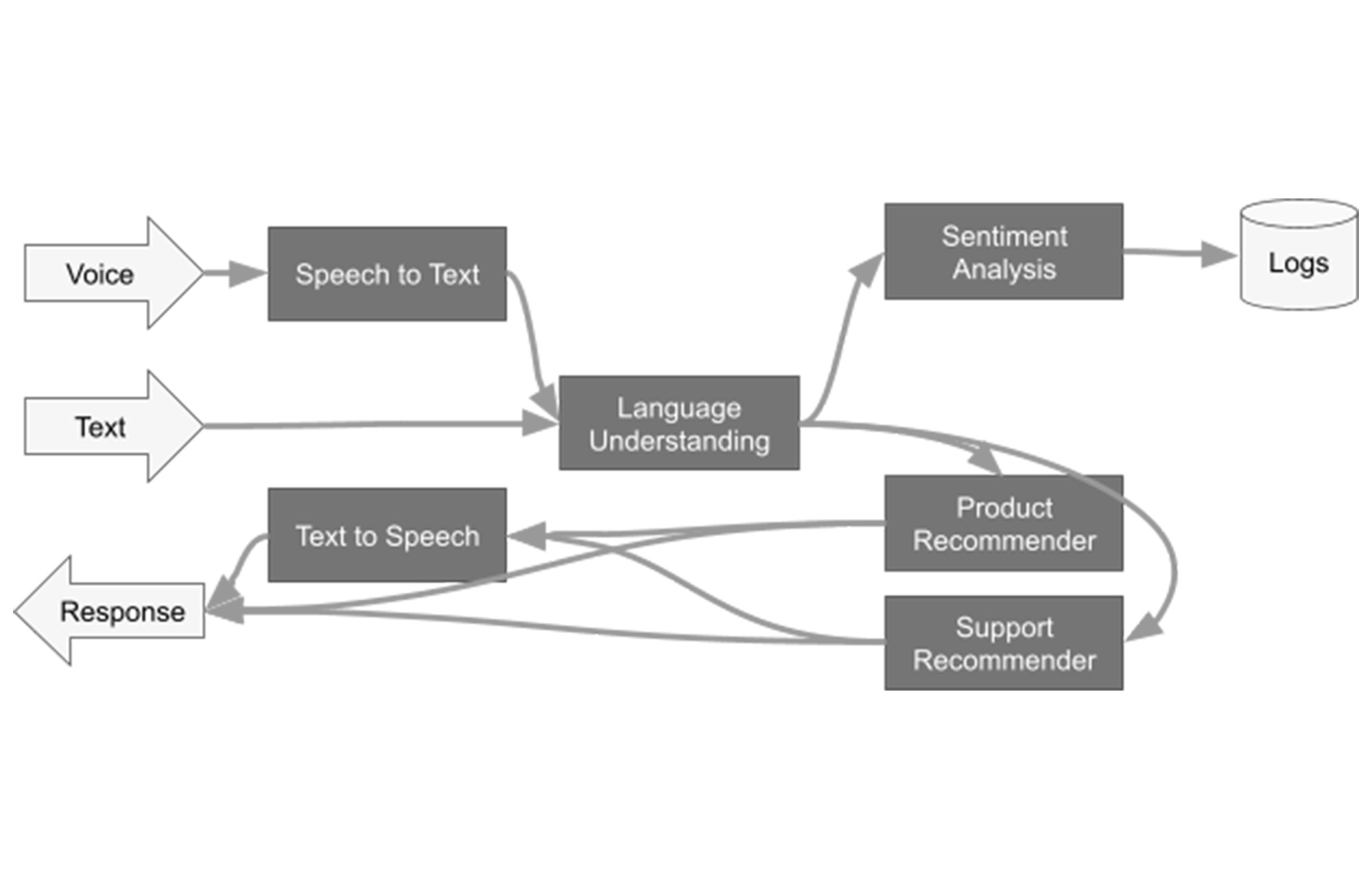
In the previous example, we had one model, a source, and an output. That pattern will be used by many pipelines. However, business needs also require ensembles of models where models are used for pre-processing of the data and for the domain specific tasks. For example, conversion of speech to text before being passed to an NLP model. Though the diagram above is a complex flow, there are actually three primary patterns.
1- Data is flowing down the graph.
2- Data can branch after a stage, for example after 'Language Understanding'.
3- Data can flow from one model into another.
Item 1 means that this is a good fit for building into a single Beam pipeline because it’s acyclic. For items 2 and 3, the Beam SDK can express the code very simply. Let’s take a look at these.
Branching Pattern:
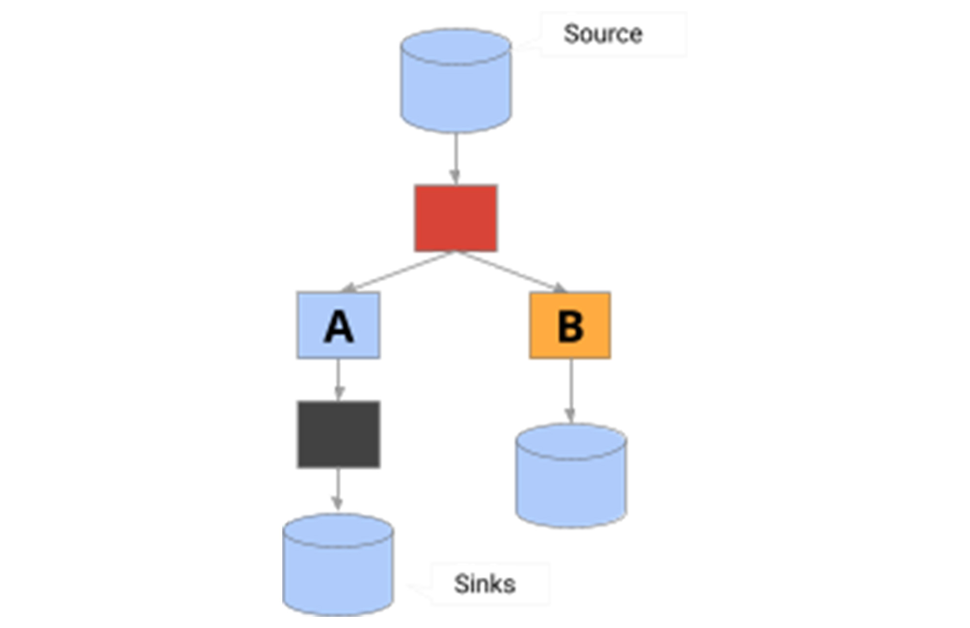
In this pattern, data is branched to two models. To send all the data to both models, the code is in the form:
Models in Sequence:
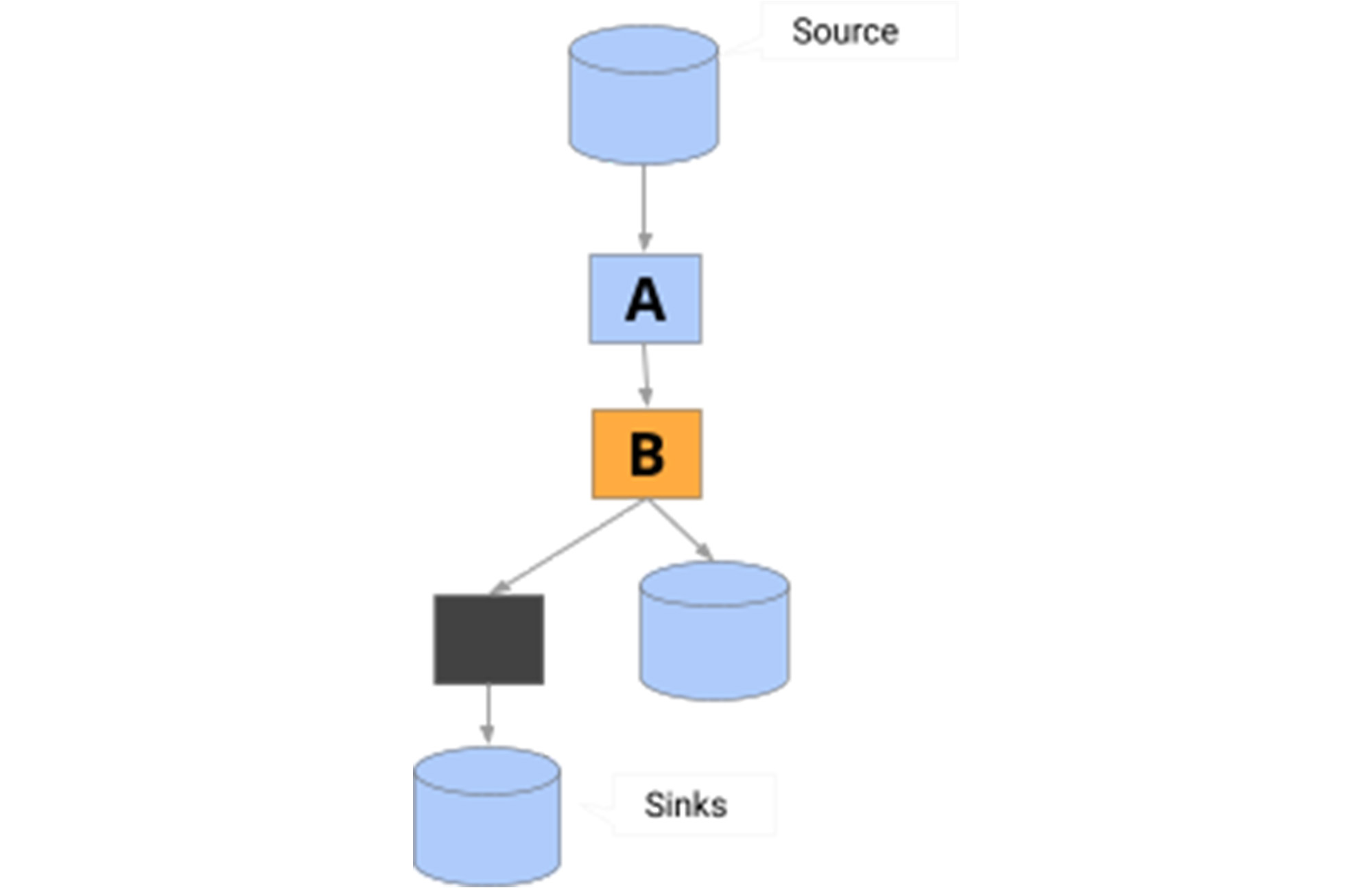
In this pattern, the output of the first model is sent to the next model. Some form of post processing normally occurs between these stages. To get the data in the right shape for the next step, the code is in the form:
With those two simple patterns (branching and model in sequence) as building blocks, we see that it’s possible to build complex ensembles of models. You can also make use of other Apache Beam tools to enrich the data at various stages in these pipelines. For example, in a sequential model, you may want to join the output of model a with data from a database before passing it to model b, bread and butter work for Beam.
Using an open source model
In the first example, we used a toy model that was available in the codelab. In this section, we walk through how you could use an open source model and output the model data to a Data Warehouse (Google Cloud BigQuery) to show a more complete end-to-end pipeline.
Note that the code in this section is self-contained and not part of the codelab used in the previous section.
The PyTorch model we will use to demonstrate this is maskrcnn_resnet50_fpn, which comes with Torchvision v 0.12.0. This model attempts to solve the image segmentation task: given an image, it detects and delineates each distinct object appearing in that image with a bounding box.
In general, libraries like Torchvision pretrained models download the pretrained model directly into memory. To run the model with RunInference, we need a different setup, because RunInference will load the model once per Python process to be shared amongst many threads. So if we want to use a pre-trained model from these types of libraries, we have a little bit of setup to do. For this PyTorch model we need to:
1- Download the state dictionary and make it available independently of the library to Beam.
2- Determine the model class file and provide it to our ModelHandler, ensuring that we disable the class’s 'autoload' features.
When looking at the signature for this model with version 0.12.0, note that there are two parameters that initiate an auto-download: pretrained and pretrained_backbone. Ensure these are both set to False to make sure that the model class does not load the model files:
model_params = {'pretrained': False, 'pretrained_backbone': False}
Step 1 -
Download the state dictionary. The location can be found in the maskrcnn_resnet50_fpn source code:
Next, push this model from the local directory where it was downloaded to a common area accessible to workers. You can use utilities like gsutil if using Google Cloud Storage (GCS) as your object store:
Step 2 -
For our Modelandler, we need to use the model_class, which in our case is torchvision.models.detection.maskrcnn_resnet50_fpn.
We can now build our ModelHandler. Note that in this case, we are making a KeyedModelHandler, which is different from the simple example we used above. The KeyedModelHandler is used to indicate that the values coming into the RunInference API are a tuple, where the first value is a key and the second is the tensor that will be used by the model. This allows us to keep a reference of which image the inference is associated with, and it is used in our post processing step.
All models need some level of pre-processing. Here we create a preprocessing function ready for our pipeline. One important note: when batching, the PyTorch ModelHandler will need the size of the tensor to be the same across the batch, so here we set the image_size as part of the pre-processing step. Also note that this function accepts a tuple with the first element being a string. This will be the 'key', and in the pipeline code, we will use the filename as the key.
The output of the model needs some post processing before being sent to BigQuery. Here we denormalise the label with the actual name, for example, person, and zip it up with the bounding box and score output:
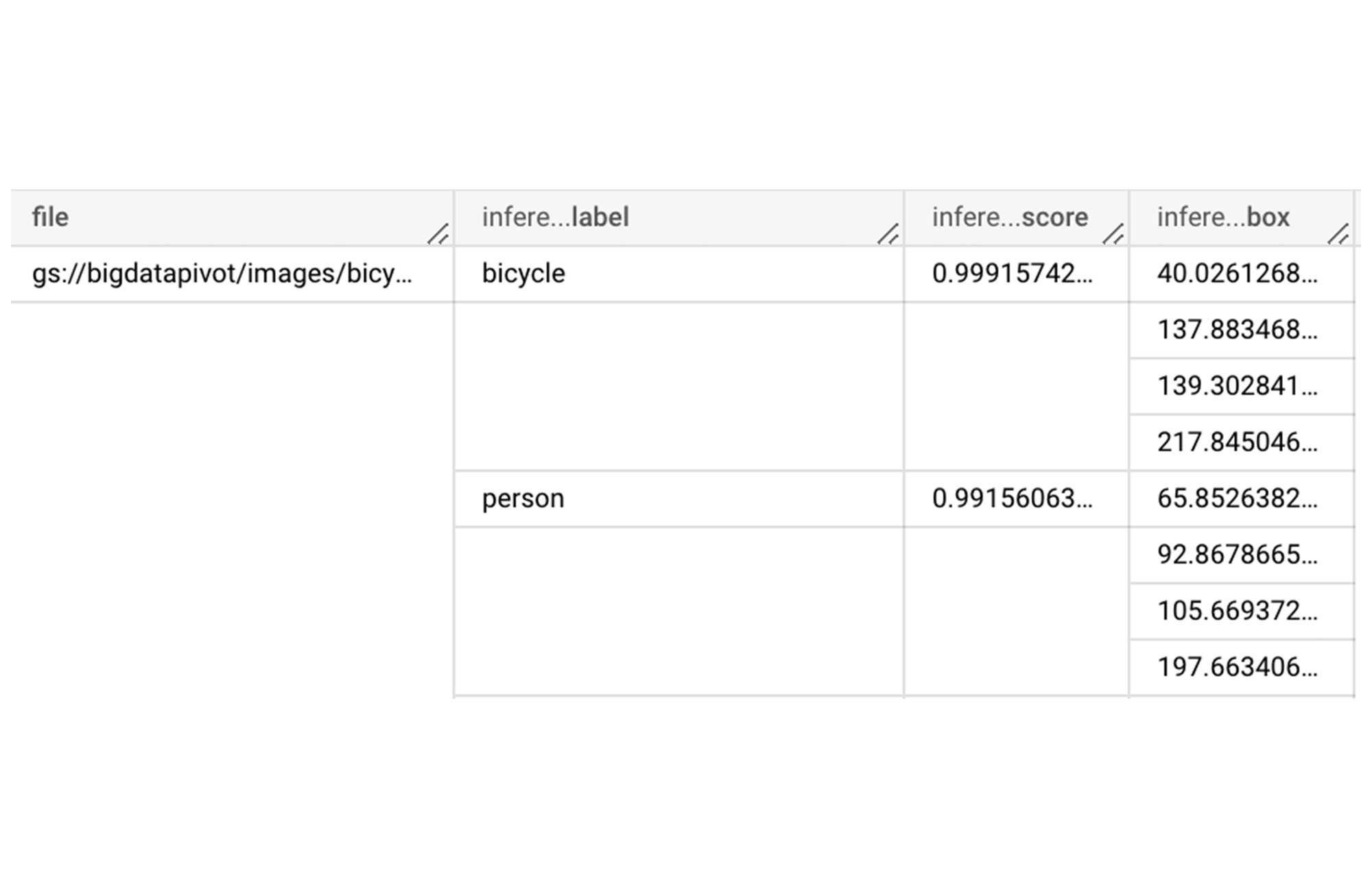
Let’s now run this pipeline with the direct runner, which will read the image from GCS, run it through the model, and output the results to BigQuery. We will need to pass in the BigQuery schema that we want to use, which should match the dict that we created in our post-processing. The WriteToBigquery transform takes the schema information as the table_spec object, which represents the following schema:
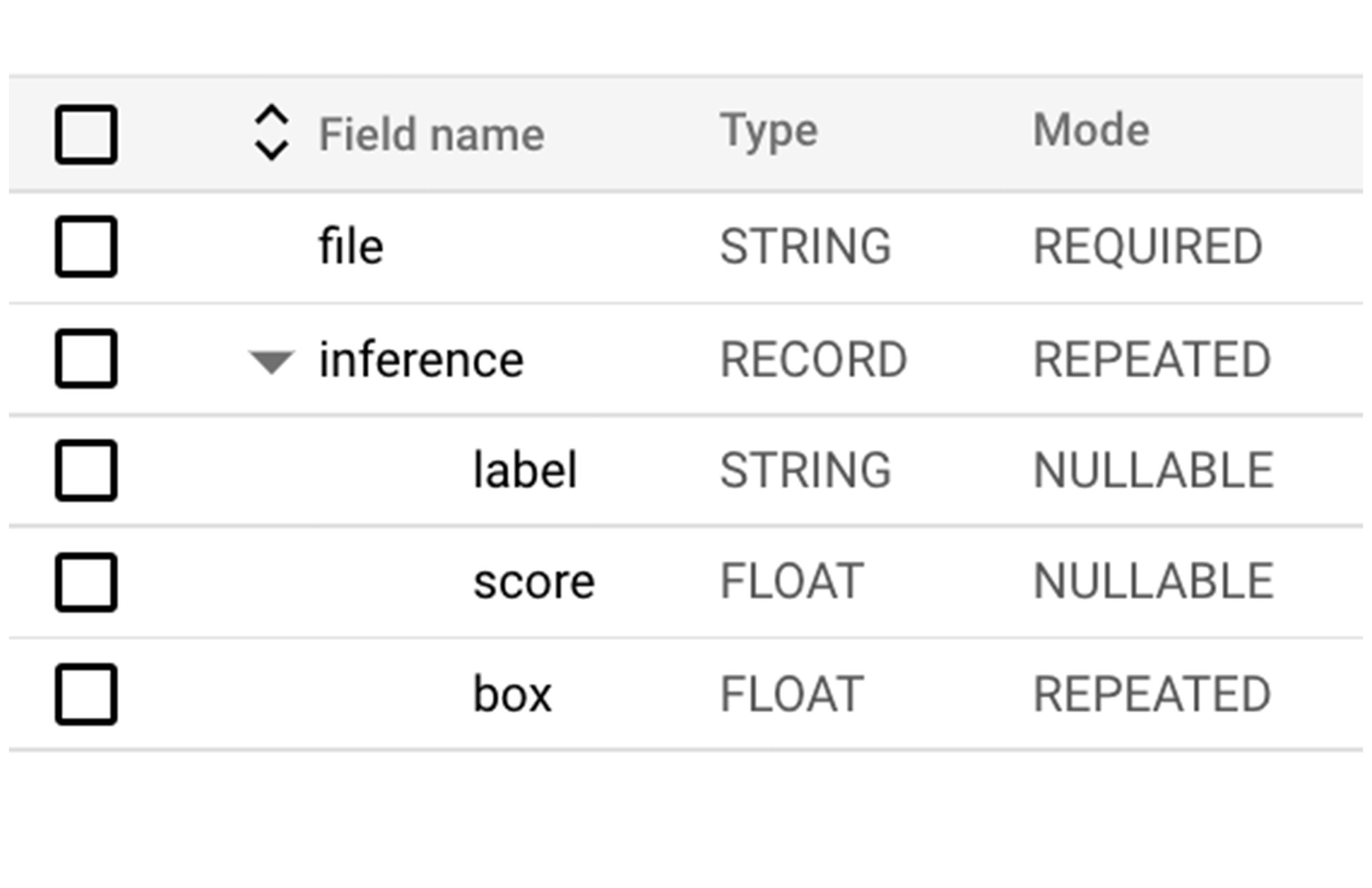
The schema has a file string, which is the key from our output tuple. Because each image's prediction will have a List of (labels, score, and bounding box points), a RECORD type is used to represent the data in BigQuery.
Next, let’s create the pipeline using pipeline options, which will use the local runner to process an image from the bucket and push it to BigQuery. Because we need access to a project for the BigQuery calls, we will pass in project information via the options:
Next, we will see the pipeline put together with pre- and post-processing steps.
The Beam transform MatchFiles matches all of the files found with the glob pattern provided. These matches are sent to the ReadMatches transform, which outputs a PCollection of ReadableFile objects. These have the Metadata.path information and can have the read() function invoked to get the files bytes(). These are then sent to the preprocessing path.
After running this pipeline, the BigQuery table will be populated with the results of the prediction.
In order to run this pipeline on the cloud, for example if we had a bucket of 10000's of images, we simply need to update the pipeline options and provide Dataflow with dependency information.:
Create requirements.txt file for the dependencies:
Creating the right pipeline options:
Conclusion
The use of the new Apache Beam apache_beam.ml.RunInference transform removes large chunks of boiler plate data pipelines that incorporate machine learning models. Pipelines that make use of these transforms will also be able to make full use of the expressiveness of Apache Beam to deal with the pre- and post-processing of the data, and build complex multi-model pipelines with minimal code.