Building ML models for everyone: understanding fairness in machine learning
Sara Robinson
Staff Developer Relations Engineer
Fairness in data, and machine learning algorithms is critical to building safe and responsible AI systems from the ground up by design. Both technical and business AI stakeholders are in constant pursuit of fairness to ensure they meaningfully address problems like AI bias. While accuracy is one metric for evaluating the accuracy of a machine learning model, fairness gives us a way to understand the practical implications of deploying the model in a real-world situation.
Fairness is the process of understanding bias introduced by your data, and ensuring your model provides equitable predictions across all demographic groups. Rather than thinking of fairness as a separate initiative, it’s important to apply fairness analysis throughout your entire ML process, making sure to continuously reevaluate your models from the perspective of fairness and inclusion. This is especially important when AI is deployed in critical business processes, like credit application reviews and medical diagnosis, that affect a wide range of end users.
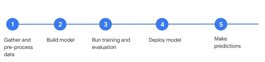
For example, the following is a typical ML lifecycle:
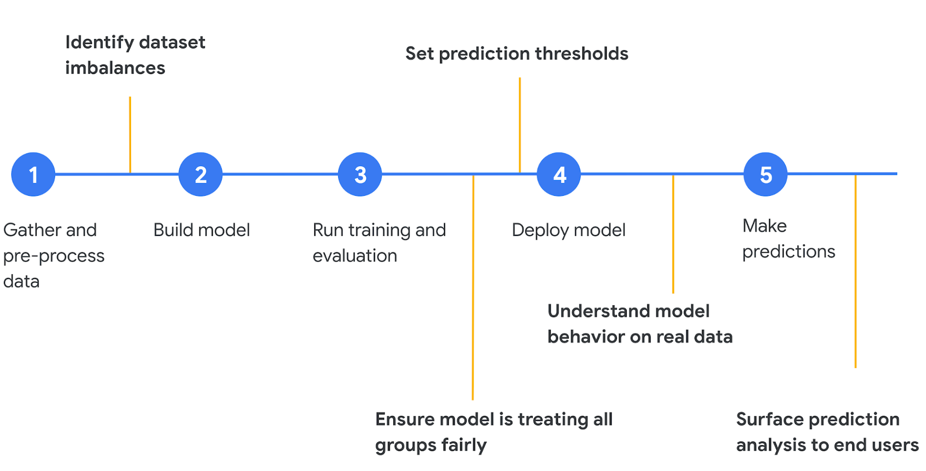
Below, in yellow, are some ways ML fairness can be applied at various stages of your model development:
Instead of thinking of a deployed model as the end of the process, think of the steps outlined above as a cycle where you’re continually evaluating the fairness of your model, adding new training data, and re-training. Once the first version of your model is deployed, it’s best to gather feedback on how the model is performing and take steps to improve its fairness in the next iteration.
In this blog we’ll focus on the first three fairness steps in the diagram above: identifying dataset imbalances, ensuring fair treatment of all groups, and setting prediction thresholds. To give you concrete methods for analyzing your models from a fairness perspective, we’ll use the What-if Tool on models deployed on AI Platform. We’ll specifically focus on the What-if Tool’s Fairness & Performance tab, which allows you to slice your data by individual features to see how your model behaves on different subsets.
We’ll be using this housing dataset from Kaggle throughout this post to show you how to perform fairness analysis in the What-if Tool. As you can see in the preview below, it includes many pieces of data on a house (square feet, number of bedrooms, kitchen quality, etc.) along with its sale price. In this exercise, we’ll be predicting whether a house will sell for more or less than $160k.
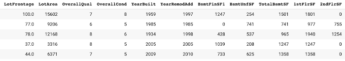
While the features here are specific to housing, the goal of this post is to help you think about how you can apply these concepts to your own dataset, which is especially important when the dataset deals with people.
Identifying dataset imbalances
Before you even start building a model, you can use the What-if Tool to better understand dataset imbalances and see where you might need to add more examples. With the following snippet, we’ll load the housing data as a Pandas DataFrame into the What-if Tool:When the visualization loads, navigate to the Features tab (note that we’ve done some pre-processing to turn categorical columns into Pandas dummy columns):
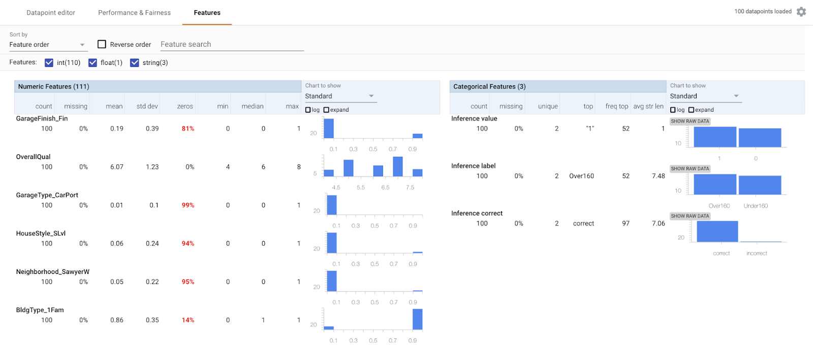
Here are some things we want to be aware of in this dataset:
This dataset is relatively small, with 1,460 total examples. It was originally intended as a regression problem, but nearly every regression problem can be converted to classification. To highlight more What-if Tool features, we turned it into a classification problem to predict whether a house is worth more or less than $160k.
Since we’ve converted it to a classification problem, we purposely chose the $160k threshold to make the label classes as balanced as possible—there are 715 houses less than $160k and 745 worth more than $160k. Real world datasets are not always so balanced.
The houses in this dataset are all in Ames, Iowa and the data was collected between 2006 and 2010. No matter what accuracy our model achieves, it wouldn’t be wise to try generating a prediction on a house in an entirely different metropolitan area, like New York City.
Similar to the point above, the ”Neighborhood” column in this data is not entirely balanced—North Ames has the most houses (225) and College Circle is next with 150.
There may also be missing data that could improve our model. For example, the original dataset includes data on a house’s basement type and size which we’ve left out of this analysis. Additionally, what if we had data on the previous residents of each house? It’s important to think about all possible data sources, even if it will require some feature engineering before feeding it into the model.
It’s best to do this type of dataset analysis before you start training a model so you can optimize the dataset and be aware of potential bias and how to account for it. Once your dataset is ready, you can build and train your model and connect it to the What-if Tool for more in-depth fairness analysis.
Connecting your AI Platform model to the What-if Tool
We’ll use XGBoost to build our model, and you can find the full code on GitHub and AI Hub.Training an XGBoost model and deploying it to AI Platform is simple:
Now that we’ve got a deployed model, we can connect it to the What-if Tool:
Running the code above should result in the following visualization:
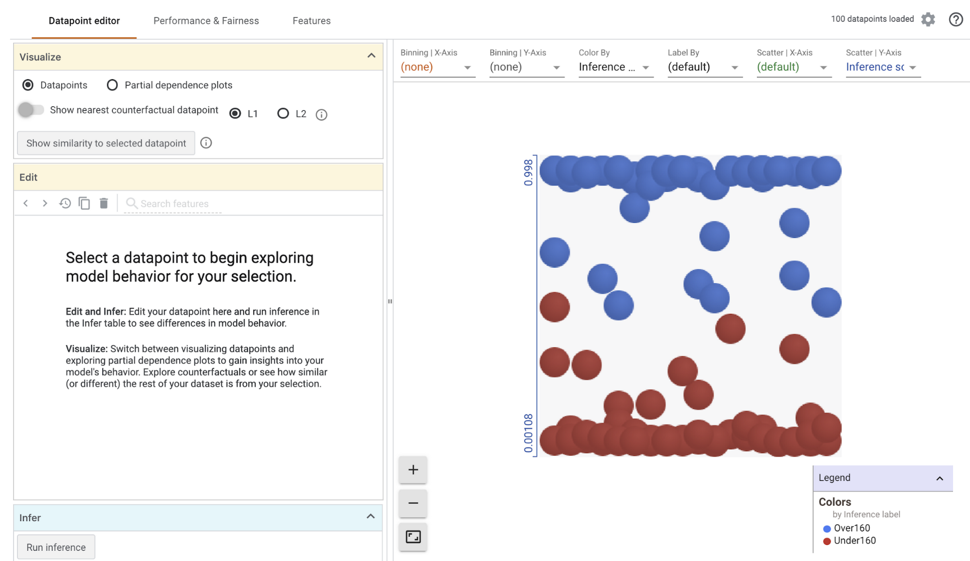
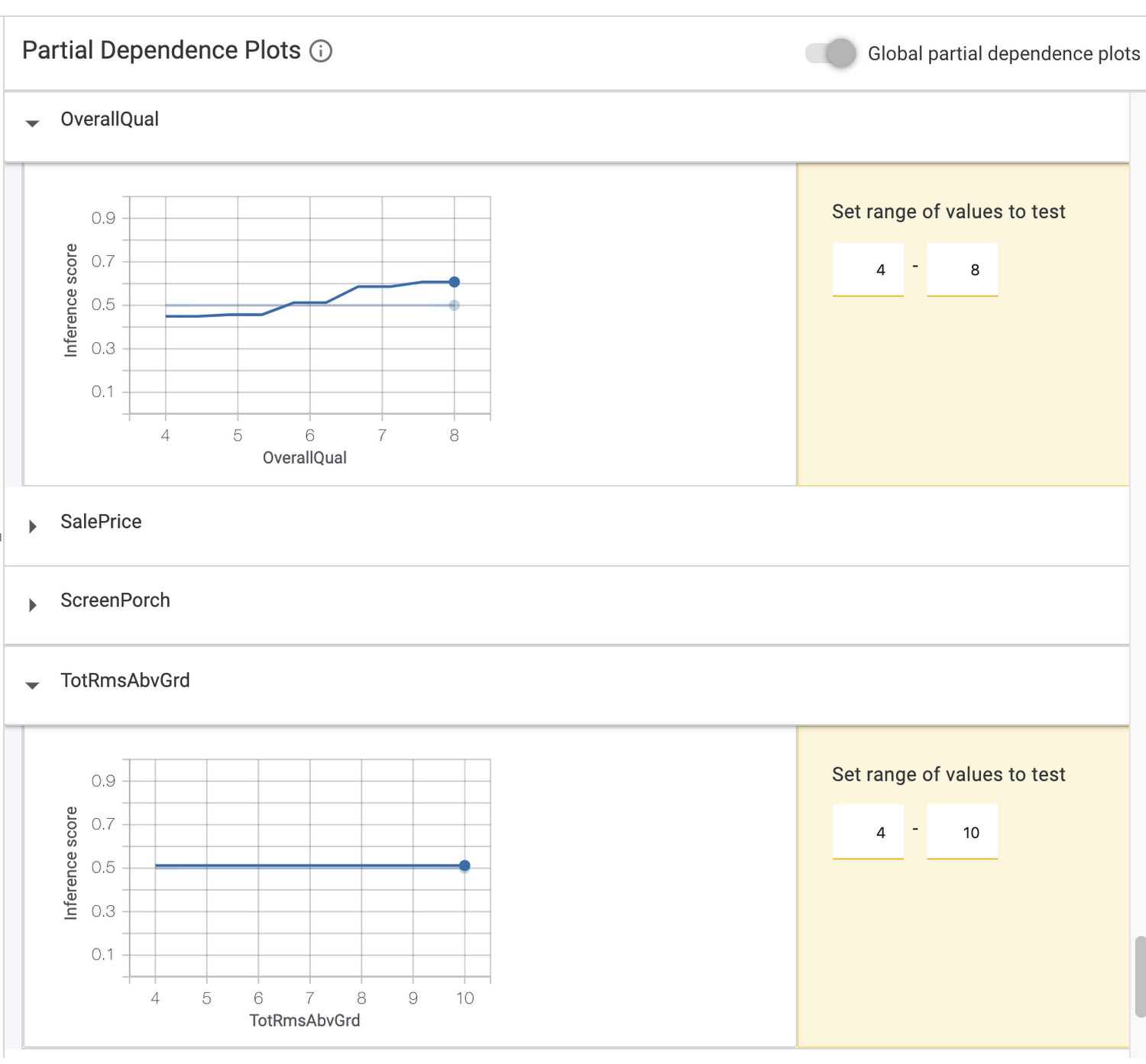
If you select Partial dependence plots on the top left, you can see how individual features impact the model’s prediction for an individual data point (if you have one selected), or globally across all data points. In the global dependence plots here, we can see that the overall quality rating of a house had a significant effect on the model’s prediction (price increases as quality rating increases) but the number of bedrooms above ground did not:
For the rest of this post we’ll focus on fairness metrics.
Getting started with the Fairness tab
On the top left of the visualization, select the Performance & Fairness tab. This is what you’ll see first: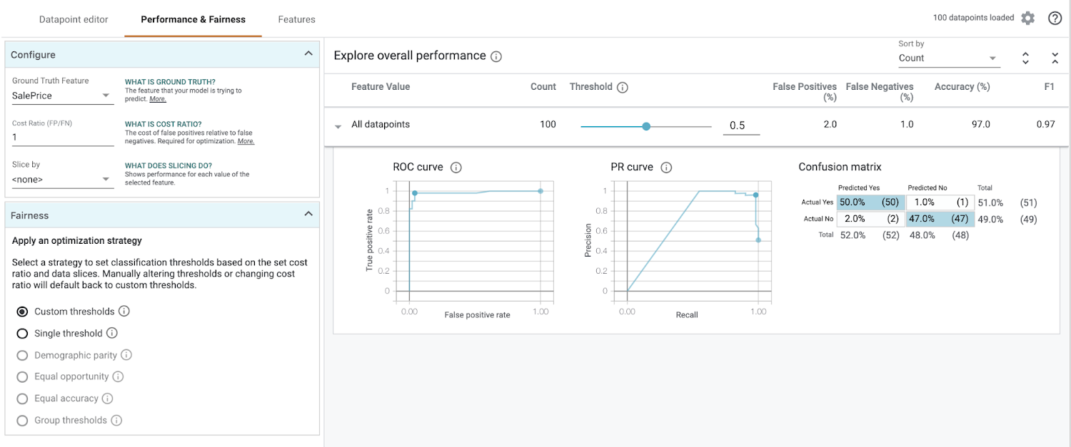
There’s a lot going on! Let’s break down what we’re looking at before we add any configuration options.
In the “Explore overall performance” section, we can see various metrics related to our model’s accuracy. By default the Threshold slider starts at 0.5. This means that our model will classify any prediction value above 0.5 as over $160k, and anything less than 0.5 will be classified as less than $160k. The threshold is something you need to determine after you’ve trained your model, and the What-if Tool can help you determine the best threshold value based on what you want to optimize for (more on that later). When you move the threshold slider you’ll notice that all of the metrics change:
The confusion matrix tells us the percentage of correct predictions for each class (the four squares add up to 100%). ROC and Precision / Recall (PR) are also common metrics for model accuracy. We’ll get the best insights from this tab once we start slicing our data.
Applying optimization strategies to data slices
In the Configure section in the top left of the What-if Tool, select a feature from the Slice by dropdown. First, let’s look at “GarageType_Attchd”, which indicates whether the garage is attached to the house (0 for no, 1 for yes):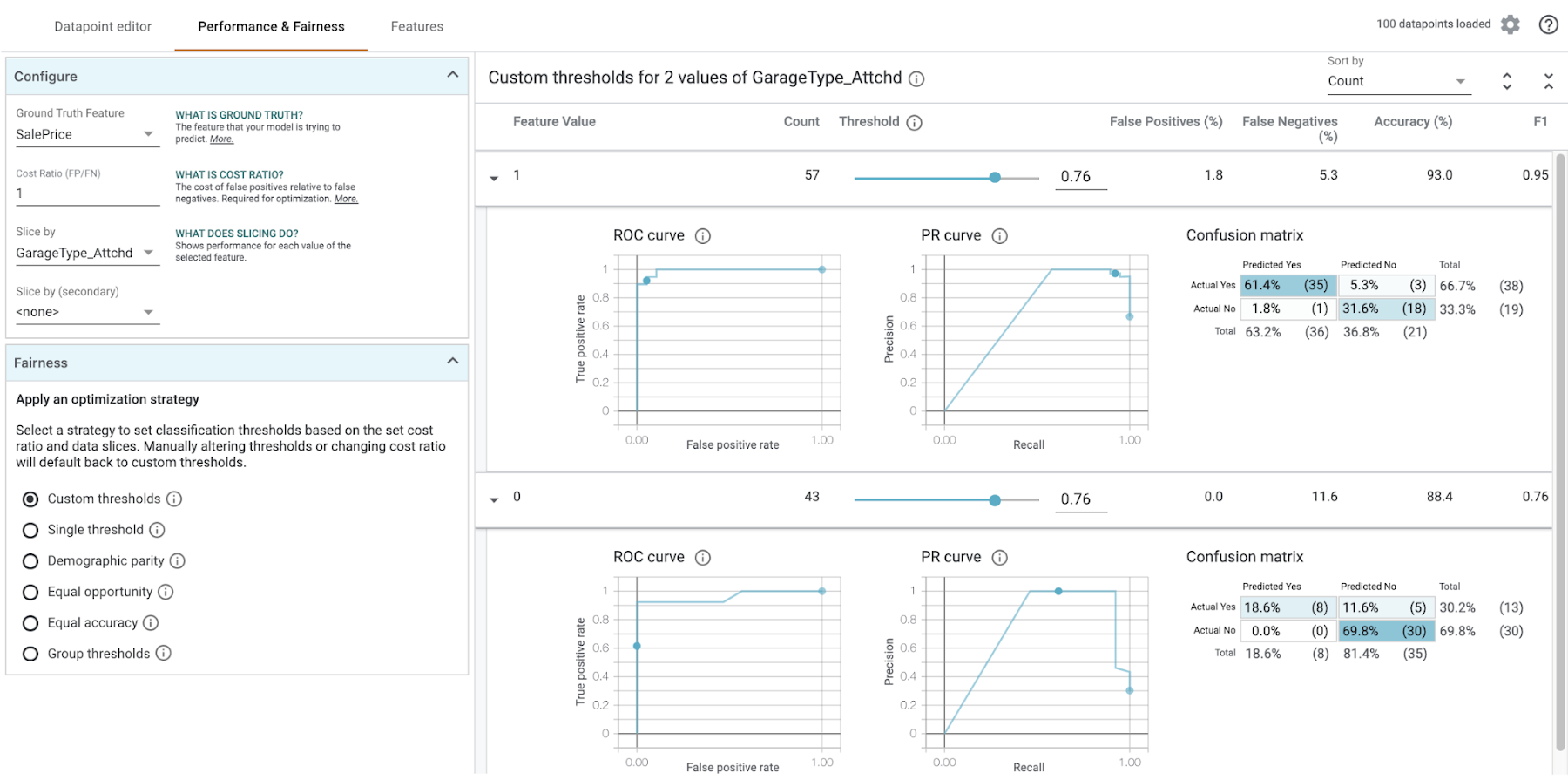
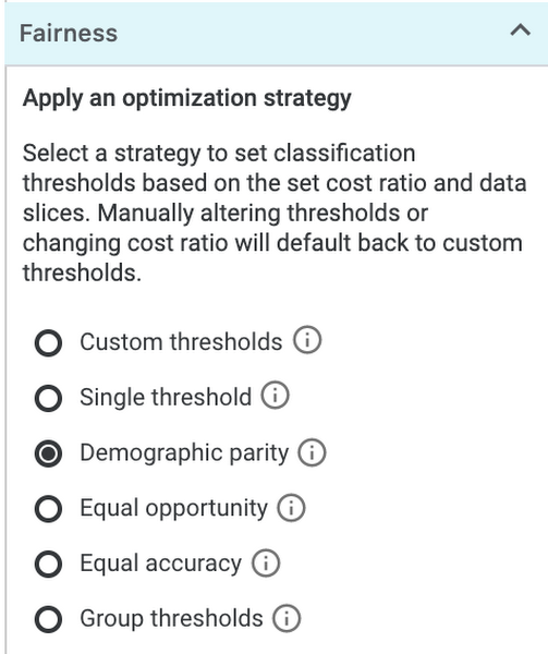
Notice that houses with an attached garage have a higher likelihood that our model will value them at more than $160k. In this case the data has already been collected, but let’s imagine that we wanted our model to price houses with attached and unattached garages in the same way. In this example we care most about having the same percentage of positive classifications across classes, while still achieving the highest possible accuracy within that constraint. For this we should select Demographic parity from the Fairness section on the bottom left:
You’ll notice that our threshold sliders and accuracy metrics change when we set this strategy:
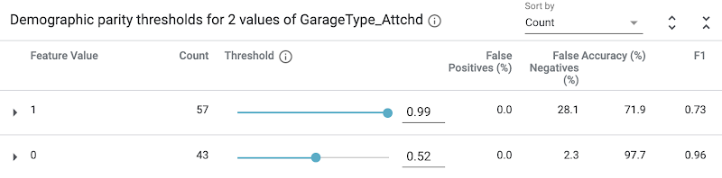
What do all these changes mean? If we don’t want the garage placement to influence our model’s price, we need to use different thresholds for houses depending on whether their garage is attached. With these updated thresholds, the model will predict the house to be worth over $160k when the prediction score is .99 or higher. Alternatively, a house without an attached garage should be classified as over $160k if the model predicts 0.52 or higher.
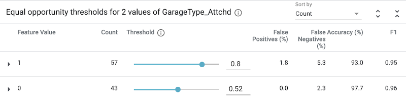
If we instead use the “Equal opportunity” strategy, it will optimize for high accuracy predictions within the positive class and ensure an equal true positive rate across data slices. In other words, this will choose the thresholds that ensure houses that are likely worth over $160k are given a fair chance of being classified for that outcome by our model. The results here are quite different:
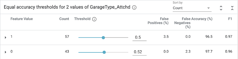
Finally, the “Equal accuracy” strategy will optimize for accuracy across both classes (positive and negative). Again, the resulting thresholds are different from either of the outcomes above:
We can do a similar slice analysis for other features, like neighborhood and house type, or we can do an intersectional analysis by slicing by two features at the same time. It’s also important to note that there are many definitions of the fairness constraints used in the What-if Tool; the ones you should use largely depend on the context of your model.
Takeaways
We used the housing dataset in our demo, but this could be applied to any type of classification task. What can we learn from doing this type of analysis? Let’s take a step back and think about what would have happened if we had not done a fairness analysis and deployed our model using a 0.5 classification threshold for all feature values. Due to biases in our training data, our model would be treating houses differently based on their location, age, size, and other features. Perhaps we want our model to behave this way for specific features (i.e. price bigger houses higher), but in other cases we’d like to adjust for this bias. Armed with the knowledge of how our model is making decisions, we can now tackle this bias by adding more balanced training data, adjusting our training loss function, or adjusting prediction thresholds to account for the type of fairness we want to work towards.Here are some more ML fairness resources that are worth checking out:
ML Fairness section in the Google’s Machine Learning Crash Course
Google I/O talk on ML Fairness
Code for the housing demo shown in this post in GitHub and AI Hub
Is there anything else you’d like to see covered on the topics of ML fairness or explainability? Let me know what you think on Twitter at @SRobTweets.