Create machine learning models in BigQuery ML

Create machine learning models in BigQuery ML

This tutorial introduces users to BigQuery ML using the Google Cloud console.

BigQuery ML enables users to create and execute machine learning models in BigQuery by using SQL queries and Python code. The goal is to democratize machine learning by enabling SQL practitioners to build models using their existing tools and to increase development speed by eliminating the need for data movement.

In this tutorial, you use the sample Google Analytics sample dataset for BigQuery to create a model that predicts whether a website visitor will make a transaction. For information on the schema of the Analytics dataset, see BigQuery export schema in the Analytics Help Center.

Objectives

In this tutorial, you use:

• BigQuery ML to create a binary logistic regression model using the CREATE MODEL statement
• The ML.EVALUATE function to evaluate the ML model
• The ML.PREDICT function to make predictions using the ML model

Costs

This tutorial uses billable components of Google Cloud, including the following:

• BigQuery
• BigQuery ML

For more information on BigQuery costs, see the BigQuery pricing page.

For more information on BigQuery ML costs, see BigQuery ML pricing.

Before you begin

1. Sign in to your Google Cloud account. If you're new to Google Cloud, create an account to evaluate how our products perform in real-world scenarios. New customers also get $300 in free credits to run, test, and deploy workloads.

2. In the Google Cloud console, on the project selector page, select or create a Google Cloud project.

   Note: If you don't plan to keep the resources that you create in this procedure, create a project instead of selecting an existing project. After you finish these steps, you can delete the project, removing all resources associated with the project.

   Go to project selector

3. Make sure that billing is enabled for your Google Cloud project.

4. In the Google Cloud console, on the project selector page, select or create a Google Cloud project.

   Note: If you don't plan to keep the resources that you create in this procedure, create a project instead of selecting an existing project. After you finish these steps, you can delete the project, removing all resources associated with the project.

   Go to project selector

5. Make sure that billing is enabled for your Google Cloud project.

6. BigQuery is automatically enabled in new projects. To activate BigQuery in a pre-existing project, go to

   Enable the BigQuery API.

   Enable the API

Create your dataset

Create a BigQuery dataset to store your ML model:

1. In the Google Cloud console, go to the BigQuery page.

   Go to the BigQuery page

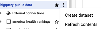
2. In the Explorer pane, click your project name.

3. Click View actions > Create dataset.

   

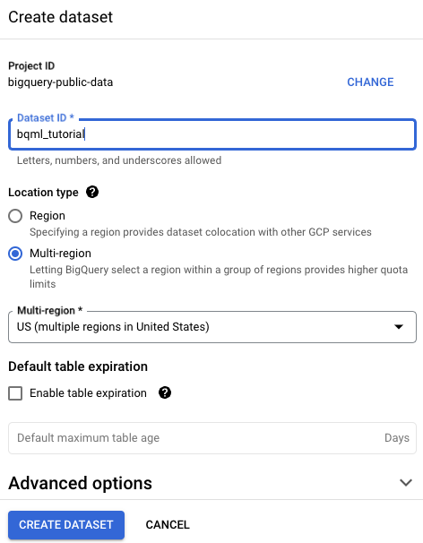
4. On the Create dataset page, do the following:

   • For Dataset ID, enter bqml_tutorial.

   • For Location type, select Multi-region, and then select US (multiple regions in United States).

     The public datasets are stored in the US multi-region. For simplicity, store your dataset in the same location.

   • Leave the remaining default settings as they are, and click Create dataset.

     

Create your model

Next, you create a logistic regression model using the Analytics sample dataset for BigQuery.

SQL

The following GoogleSQL query is used to create the model you use to predict whether a website visitor will make a transaction.

#standardSQL
CREATE MODEL `bqml_tutorial.sample_model`
OPTIONS(model_type='logistic_reg') AS
SELECT
IF(totals.transactions IS NULL, 0, 1) AS label,
IFNULL(device.operatingSystem, "") AS os,
device.isMobile AS is_mobile,
IFNULL(geoNetwork.country, "") AS country,
IFNULL(totals.pageviews, 0) AS pageviews
FROM
`bigquery-public-data.google_analytics_sample.ga_sessions_*`
WHERE
_TABLE_SUFFIX BETWEEN '20160801' AND '20170630'

In addition to creating the model, running a query that contains the CREATE MODEL statement trains the model using the data retrieved by your query's SELECT statement.

Query details

The CREATE MODEL clause is used to create and train the model named bqml_tutorial.sample_model.

The OPTIONS(model_type='logistic_reg') clause indicates that you are creating a logistic regression model. A logistic regression model tries to split input data into two classes and gives the probability the data is in one of the classes. Usually, what you are trying to detect (such as whether an email is spam) is represented by 1 and everything else is represented by 0. If the logistic regression model outputs 0.9, there is a 90% probability the input is what you are trying to detect (the email is spam).

This query's SELECT statement retrieves the following columns that are used by the model to predict the probability a customer will complete a transaction:

• totals.transactions — The total number of ecommerce transactions within the session. If the number of transactions is NULL, the value in the label column is set to 0. Otherwise, it is set to 1. These values represent the possible outcomes. Creating an alias named label is an alternative to setting the input_label_cols= option in the CREATE MODEL statement.
• device.operatingSystem — The operating system of the visitor's device.
• device.isMobile — Indicates whether the visitor's device is a mobile device.
• geoNetwork.country — The country from which the sessions originated, based on the IP address.
• totals.pageviews — The total number of page views within the session.

The FROM clause — bigquery-public-data.google_analytics_sample.ga_sessions_* — indicates that you are querying the Google Analytics sample dataset. This dataset is in the bigquery-public-data project. You are querying a set of tables sharded by date. This is represented by the wildcard in the table name: google_analytics_sample.ga_sessions_*.

The WHERE clause — _TABLE_SUFFIX BETWEEN '20160801' AND '20170630' — limits the number of tables scanned by the query. The date range scanned is August 1, 2016 to June 30, 2017.

Run the CREATE MODEL query

To run the CREATE MODEL query to create and train your model:

1. In the Google Cloud console, click the Compose new query button. If this text is unavailable to click, then the Query editor is already open.

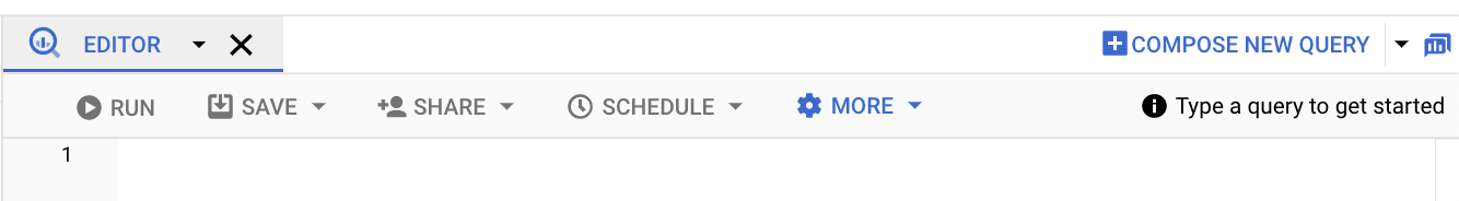
1. Enter the following GoogleSQL query in the Query editor text area.

   #standardSQL
   CREATE MODEL `bqml_tutorial.sample_model`
   OPTIONS(model_type='logistic_reg') AS
   SELECT
   IF(totals.transactions IS NULL, 0, 1) AS label,
   IFNULL(device.operatingSystem, "") AS os,
   device.isMobile AS is_mobile,
   IFNULL(geoNetwork.country, "") AS country,
   IFNULL(totals.pageviews, 0) AS pageviews
   FROM
   `bigquery-public-data.google_analytics_sample.ga_sessions_*`
   WHERE
   _TABLE_SUFFIX BETWEEN '20160801' AND '20170630'
   

2. Click Run.

   The query takes several minutes to complete. After the first iteration is complete, your model (sample_model) appears in the navigation panel. Because the query uses a CREATE MODEL statement to create a model, you do not see query results.

   You can observe the model as it's being trained by viewing the Model stats tab. As soon as the first iteration completes, the tab is updated. The stats continue to update as each iteration completes.

BigQuery DataFrames

Before trying this sample, follow the BigQuery DataFrames setup instructions in the BigQuery quickstart using BigQuery DataFrames. For more information, see the BigQuery DataFrames reference documentation.

To authenticate to BigQuery, set up Application Default Credentials. For more information, see Set up authentication for a local development environment.

from bigframes.ml.linear_model import LogisticRegression
import bigframes.pandas as bpd

# Start by selecting the data you'll use for training. `read_gbq` accepts
# either a SQL query or a table ID. Since this example selects from multiple
# tables via a wildcard, use SQL to define this data. Watch issue
# https://github.com/googleapis/python-bigquery-dataframes/issues/169
# for updates to `read_gbq` to support wildcard tables.

df = bpd.read_gbq_table(
    "bigquery-public-data.google_analytics_sample.ga_sessions_*",
    filters=[
        ("_table_suffix", ">=", "20160801"),
        ("_table_suffix", "<=", "20170630"),
    ],
)

# Extract the total number of transactions within
# the Google Analytics session.
#
# Because the totals column is a STRUCT data type, call
# Series.struct.field("transactions") to extract the transactions field.
# See the reference documentation below:
# https://cloud.google.com/python/docs/reference/bigframes/latest/bigframes.operations.structs.StructAccessor#bigframes_operations_structs_StructAccessor_field
transactions = df["totals"].struct.field("transactions")

# The "label" values represent the outcome of the model's
# prediction. In this case, the model predicts if there are any
# ecommerce transactions within the Google Analytics session.
# If the number of transactions is NULL, the value in the label
# column is set to 0. Otherwise, it is set to 1.
label = transactions.notnull().map({True: 1, False: 0}).rename("label")

# Extract the operating system of the visitor's device.
operating_system = df["device"].struct.field("operatingSystem")
operating_system = operating_system.fillna("")

# Extract whether the visitor's device is a mobile device.
is_mobile = df["device"].struct.field("isMobile")

# Extract the country from which the sessions originated, based on the IP address.
country = df["geoNetwork"].struct.field("country").fillna("")

# Extract the total number of page views within the session.
pageviews = df["totals"].struct.field("pageviews").fillna(0)

# Combine all the feature columns into a single DataFrame
# to use as training data.
features = bpd.DataFrame(
    {
        "os": operating_system,
        "is_mobile": is_mobile,
        "country": country,
        "pageviews": pageviews,
    }
)

# Logistic Regression model splits data into two classes, giving the
# a confidence score that the data is in one of the classes.
model = LogisticRegression()
model.fit(features, label)

# The model.fit() call above created a temporary model.
# Use the to_gbq() method to write to a permanent location.
model.to_gbq(
    your_model_id,  # For example: "bqml_tutorial.sample_model",
    replace=True,
)

Get training statistics

To see the results of the model training, you can use the ML.TRAINING_INFO function, or you can view the statistics in the Google Cloud console. In this tutorial, you use the Google Cloud console.

Machine learning is about creating a model that can use data to make a prediction. The model is essentially a function that takes inputs and applies calculations to the inputs to produce an output — a prediction.

Machine learning algorithms work by taking several examples where the prediction is already known (such as the historical data of user purchases) and iteratively adjusting various weights in the model so that the model's predictions match the true values. It does this by minimizing how wrong the model is using a metric called loss.

The expectation is that for each iteration, the loss should be decreasing (ideally to zero). A loss of zero means the model is 100% accurate.

To see the model training statistics that were generated when you ran the CREATE MODEL query:

1. In the navigation panel of the Google Cloud console, in the Resources section, expand [PROJECT_ID] > bqml_tutorial and then click sample_model.

2. Click the Model stats tab. The results should look like the following:

   

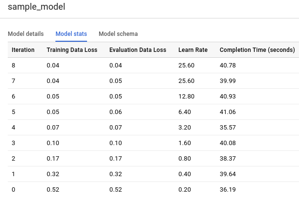
   The Training Data Loss column represents the loss metric calculated after the given iteration on the training dataset. Since you performed a logistic regression, this column is the log loss. The Evaluation Data Loss column is the same loss metric calculated on the holdout dataset (data that is held back from training to validate the model).

   BigQuery ML automatically splits your input data into a training set and a holdout set to avoid overfitting the model. This is necessary so that the training algorithm doesn't so closely tailor to the known data that it doesn't generalize to unseen, new examples.

   Training Data Loss and Evaluation Data Loss are average loss values, averaged over all examples in the respective sets.

   For more details on the ML.TRAINING_INFO function, see the BigQuery ML Syntax Reference.

Evaluate your model

After creating your model, you evaluate the performance of the classifier using the ML.EVALUATE function. The ML.EVALUATE function evaluates the predicted values against the actual data. To calculate logistic regression specific metrics, use the ML.ROC_CURVE SQL function or the bigframes.ml.metrics.roc_curve BigQuery DataFrames function.

In this tutorial you are using a binary classification model that detects transactions. The two classes are the values in the label column: 0 (no transactions) and 1 (transaction made).

SQL

The query used to evaluate the model is as follows:

#standardSQL
SELECT
*
FROM
ML.EVALUATE(MODEL `bqml_tutorial.sample_model`, (
SELECT
IF(totals.transactions IS NULL, 0, 1) AS label,
IFNULL(device.operatingSystem, "") AS os,
device.isMobile AS is_mobile,
IFNULL(geoNetwork.country, "") AS country,
IFNULL(totals.pageviews, 0) AS pageviews
FROM
`bigquery-public-data.google_analytics_sample.ga_sessions_*`
WHERE
_TABLE_SUFFIX BETWEEN '20170701' AND '20170801'))

Query details

The top-most SELECT statement retrieves the columns from your model.

The FROM clause uses the ML.EVALUATE function against your model: bqml_tutorial.sample_model.

This query's nested SELECT statement and FROM clause are the same as those in the CREATE MODEL query.

The WHERE clause — _TABLE_SUFFIX BETWEEN '20170701' AND '20170801' — limits the number of tables scanned by the query. The date range scanned is July 1, 2017 to August 1, 2017. This is the data you're using to evaluate the predictive performance of the model. It was collected in the month immediately following the time period spanned by the training data.

Run the ML.EVALUATE query

To run the ML.EVALUATE query that evaluates the model:

1. In the Google Cloud console, click the Compose new query button.

2. Enter the following GoogleSQL query in the Query editor text area.

   #standardSQL
   SELECT
   *
   FROM
   ML.EVALUATE(MODEL `bqml_tutorial.sample_model`, (
   SELECT
   IF(totals.transactions IS NULL, 0, 1) AS label,
   IFNULL(device.operatingSystem, "") AS os,
   device.isMobile AS is_mobile,
   IFNULL(geoNetwork.country, "") AS country,
   IFNULL(totals.pageviews, 0) AS pageviews
   FROM
   `bigquery-public-data.google_analytics_sample.ga_sessions_*`
   WHERE
   _TABLE_SUFFIX BETWEEN '20170701' AND '20170801'))
   

3. Click Run.

4. When the query is complete, click the Results tab below the query text area. The results should look like the following:

   +--------------------+---------------------+--------------------+--------------------+---------------------+----------+
   |     precision      |       recall        |      accuracy      |      f1_score      |      log_loss       | roc_auc  |
   +--------------------+---------------------+--------------------+--------------------+---------------------+----------+
   | 0.4451901565995526 | 0.08879964301651048 | 0.9716829479411401 | 0.1480654761904762 | 0.07921781778780206 | 0.970706 |
   +--------------------+---------------------+--------------------+--------------------+---------------------+----------+
   

   Because you performed a logistic regression, the results include the following columns:

   • precision — A metric for classification models. Precision identifies the frequency with which a model was correct when predicting the positive class.

   • recall — A metric for classification models that answers the following question: Out of all the possible positive labels, how many did the model correctly identify?

   • accuracy — Accuracy is the fraction of predictions that a classification model got right.

   • f1_score — A measure of the accuracy of the model. The f1 score is the harmonic average of the precision and recall. An f1 score's best value is 1. The worst value is 0.

   • log_loss — The loss function used in a logistic regression. This is the measure of how far the model's predictions are from the correct labels.

   • roc_auc — The area under the ROC curve. This is the probability that a classifier is more confident that a randomly chosen positive example is actually positive than that a randomly chosen negative example is positive. For more information, see Classification in the Machine Learning Crash Course.

BigQuery DataFrames

Before trying this sample, follow the BigQuery DataFrames setup instructions in the BigQuery quickstart using BigQuery DataFrames. For more information, see the BigQuery DataFrames reference documentation.

To authenticate to BigQuery, set up Application Default Credentials. For more information, see Set up authentication for a local development environment.

import bigframes.pandas as bpd

# Select model you'll use for evaluating. `read_gbq_model` loads model data from a
# BigQuery, but you could also use the `model` object from the previous steps.
model = bpd.read_gbq_model(
    your_model_id,  # For example: "bqml_tutorial.sample_model",
)

# The filters parameter limits the number of tables scanned by the query.
# The date range scanned is July 1, 2017 to August 1, 2017. This is the
# data you're using to evaluate the predictive performance of the model.
# It was collected in the month immediately following the time period
# spanned by the training data.
df = bpd.read_gbq_table(
    "bigquery-public-data.google_analytics_sample.ga_sessions_*",
    filters=[
        ("_table_suffix", ">=", "20170701"),
        ("_table_suffix", "<=", "20170801"),
    ],
)

transactions = df["totals"].struct.field("transactions")
label = transactions.notnull().map({True: 1, False: 0}).rename("label")
operating_system = df["device"].struct.field("operatingSystem")
operating_system = operating_system.fillna("")
is_mobile = df["device"].struct.field("isMobile")
country = df["geoNetwork"].struct.field("country").fillna("")
pageviews = df["totals"].struct.field("pageviews").fillna(0)
features = bpd.DataFrame(
    {
        "os": operating_system,
        "is_mobile": is_mobile,
        "country": country,
        "pageviews": pageviews,
    }
)

# Some models include a convenient .score(X, y) method for evaluation with a preset accuracy metric:

# Because you performed a logistic regression, the results include the following columns:

# - precision — A metric for classification models. Precision identifies the frequency with
# which a model was correct when predicting the positive class.

# - recall — A metric for classification models that answers the following question:
# Out of all the possible positive labels, how many did the model correctly identify?

# - accuracy — Accuracy is the fraction of predictions that a classification model got right.

# - f1_score — A measure of the accuracy of the model. The f1 score is the harmonic average of
# the precision and recall. An f1 score's best value is 1. The worst value is 0.

# - log_loss — The loss function used in a logistic regression. This is the measure of how far the
# model's predictions are from the correct labels.

# - roc_auc — The area under the ROC curve. This is the probability that a classifier is more confident that
# a randomly chosen positive example
# is actually positive than that a randomly chosen negative example is positive. For more information,
# see ['Classification']('https://developers.google.com/machine-learning/crash-course/classification/video-lecture')
# in the Machine Learning Crash Course.

model.score(features, label)
#    precision    recall  accuracy  f1_score  log_loss   roc_auc
# 0   0.412621  0.079143  0.985074  0.132812  0.049764  0.974285
# [1 rows x 6 columns]

Use your model to predict outcomes

Now that you have evaluated your model, the next step is to use it to predict an outcome. You use your model to predict the number of transactions made by website visitors from each country.

SQL

The query used to predict the outcome is as follows:

#standardSQL
SELECT
country,
SUM(predicted_label) as total_predicted_purchases
FROM
ML.PREDICT(MODEL `bqml_tutorial.sample_model`, (
SELECT
IFNULL(device.operatingSystem, "") AS os,
device.isMobile AS is_mobile,
IFNULL(totals.pageviews, 0) AS pageviews,
IFNULL(geoNetwork.country, "") AS country
FROM
`bigquery-public-data.google_analytics_sample.ga_sessions_*`
WHERE
_TABLE_SUFFIX BETWEEN '20170701' AND '20170801'))
GROUP BY country
ORDER BY total_predicted_purchases DESC
LIMIT 10

Query details

The top-most SELECT statement retrieves the country column and sums the predicted_label column. This column is generated by the ML.PREDICT function. When you use the ML.PREDICT function the output column name for the model is predicted_<label_column_name>. For linear regression models, predicted_label is the estimated value of label. For logistic regression models, predicted_label is the most likely label, which in this case is either 0 or 1.

Note: A more refined use of ML.PREDICT would sum the predicted probabilities of each label in the predicted_label_probs array. For more informations, see the ML.PREDICT syntax reference.

The ML.PREDICT function is used to predict results using your model: bqml_tutorial.sample_model.

This query's nested SELECT statement and FROM clause are the same as those in the CREATE MODEL query.

The WHERE clause — _TABLE_SUFFIX BETWEEN '20170701' AND '20170801' — limits the number of tables scanned by the query. The date range scanned is July 1, 2017 to August 1, 2017. This is the data for which you're making predictions. It was collected in the month immediately following the time period spanned by the training data.

The GROUP BY and ORDER BY clauses group the results by country and order them by the sum of the predicted purchases in descending order.

The LIMIT clause is used here to display only the top 10 results.

Run the ML.PREDICT query

To run the query that uses the model to predict an outcome:

1. In the Google Cloud console, click the Compose new query button.

2. Enter the following GoogleSQL query in the Query editor text area.

   #standardSQL
   SELECT
   country,
   SUM(predicted_label) as total_predicted_purchases
   FROM
   ML.PREDICT(MODEL `bqml_tutorial.sample_model`, (
   SELECT
   IFNULL(device.operatingSystem, "") AS os,
   device.isMobile AS is_mobile,
   IFNULL(totals.pageviews, 0) AS pageviews,
   IFNULL(geoNetwork.country, "") AS country
   FROM
   `bigquery-public-data.google_analytics_sample.ga_sessions_*`
   WHERE
   _TABLE_SUFFIX BETWEEN '20170701' AND '20170801'))
   GROUP BY country
   ORDER BY total_predicted_purchases DESC
   LIMIT 10
   

3. Click Run.

4. When the query is complete, click the Results tab below the query text area. The results should look like the following:

+----------------+---------------------------+
|    country     | total_predicted_purchases |
+----------------+---------------------------+
| United States  |                       209 |
| Taiwan         |                         6 |
| Canada         |                         4 |
| Turkey         |                         2 |
| India          |                         2 |
| Japan          |                         2 |
| Indonesia      |                         1 |
| United Kingdom |                         1 |
| Guyana         |                         1 |
+----------------+---------------------------+

BigQuery DataFrames

Before trying this sample, follow the BigQuery DataFrames setup instructions in the BigQuery quickstart using BigQuery DataFrames. For more information, see the BigQuery DataFrames reference documentation.

To authenticate to BigQuery, set up Application Default Credentials. For more information, see Set up authentication for a local development environment.

import bigframes.pandas as bpd

# Select model you'll use for predicting.
# `read_gbq_model` loads model data from
# BigQuery, but you could also use the `model`
# object from the previous steps.
model = bpd.read_gbq_model(
    your_model_id,  # For example: "bqml_tutorial.sample_model",
)

# The filters parameter limits the number of tables scanned by the query.
# The date range scanned is July 1, 2017 to August 1, 2017. This is the
# data you're using to make the prediction.
# It was collected in the month immediately following the time period
# spanned by the training data.
df = bpd.read_gbq_table(
    "bigquery-public-data.google_analytics_sample.ga_sessions_*",
    filters=[
        ("_table_suffix", ">=", "20170701"),
        ("_table_suffix", "<=", "20170801"),
    ],
)

operating_system = df["device"].struct.field("operatingSystem")
operating_system = operating_system.fillna("")
is_mobile = df["device"].struct.field("isMobile")
country = df["geoNetwork"].struct.field("country").fillna("")
pageviews = df["totals"].struct.field("pageviews").fillna(0)
features = bpd.DataFrame(
    {
        "os": operating_system,
        "is_mobile": is_mobile,
        "country": country,
        "pageviews": pageviews,
    }
)
# Use Logistic Regression predict method to predict results
# using your model.
# Find more information here in
# [BigFrames](https://cloud.google.com/python/docs/reference/bigframes/latest/bigframes.ml.linear_model.LogisticRegression#bigframes_ml_linear_model_LogisticRegression_predict)

predictions = model.predict(features)

# Call groupby method to group predicted_label by country.
# Call sum method to get the total_predicted_label by country.
total_predicted_purchases = predictions.groupby(["country"])[
    ["predicted_label"]
].sum()

# Call the sort_values method with the parameter
# ascending = False to get the highest values.
# Call head method to limit to the 10 highest values.
total_predicted_purchases.sort_values(ascending=False).head(10)

# country
# United States    220
# Taiwan             8
# Canada             7
# India              2
# Japan              2
# Turkey             2
# Australia          1
# Brazil             1
# Germany            1
# Guyana             1
# Name: predicted_label, dtype: Int64

Predict purchases per user

In this example, you try to predict the number of transactions each website visitor will make.

SQL

This query is identical to the previous query except for the GROUP BY clause. Here the GROUP BY clause — GROUP BY fullVisitorId — is used to group the results by visitor ID.

To run the query:

1. In the Google Cloud console, click the Compose new query button.

2. Enter the following GoogleSQL query in the Query editor text area.

   #standardSQL
   SELECT
   fullVisitorId,
   SUM(predicted_label) as total_predicted_purchases
   FROM
   ML.PREDICT(MODEL `bqml_tutorial.sample_model`, (
   SELECT
   IFNULL(device.operatingSystem, "") AS os,
   device.isMobile AS is_mobile,
   IFNULL(totals.pageviews, 0) AS pageviews,
   IFNULL(geoNetwork.country, "") AS country,
   fullVisitorId
   FROM
   `bigquery-public-data.google_analytics_sample.ga_sessions_*`
   WHERE
   _TABLE_SUFFIX BETWEEN '20170701' AND '20170801'))
   GROUP BY fullVisitorId
   ORDER BY total_predicted_purchases DESC
   LIMIT 10
   

3. Click Run.

4. When the query is complete, click the Results tab below the query text area. The results should look like the following:

   +---------------------+---------------------------+
   |    fullVisitorId    | total_predicted_purchases |
   +---------------------+---------------------------+
   | 9417857471295131045 |                         4 |
   | 2158257269735455737 |                         3 |
   | 5073919761051630191 |                         3 |
   | 7104098063250586249 |                         2 |
   | 4668039979320382648 |                         2 |
   | 1280993661204347450 |                         2 |
   | 7701613595320832147 |                         2 |
   | 0376394056092189113 |                         2 |
   | 9097465012770697796 |                         2 |
   | 4419259211147428491 |                         2 |
   +---------------------+---------------------------+
   

BigQuery DataFrames

Before trying this sample, follow the BigQuery DataFrames setup instructions in the BigQuery quickstart using BigQuery DataFrames. For more information, see the BigQuery DataFrames reference documentation.

To authenticate to BigQuery, set up Application Default Credentials. For more information, see Set up authentication for a local development environment.

import bigframes.pandas as bpd

# Select model you'll use for predicting.
# `read_gbq_model` loads model data from
# BigQuery, but you could also use the `model`
# object from the previous steps.
model = bpd.read_gbq_model(
    your_model_id,  # For example: "bqml_tutorial.sample_model",
)

# The filters parameter limits the number of tables scanned by the query.
# The date range scanned is July 1, 2017 to August 1, 2017. This is the
# data you're using to make the prediction.
# It was collected in the month immediately following the time period
# spanned by the training data.
df = bpd.read_gbq_table(
    "bigquery-public-data.google_analytics_sample.ga_sessions_*",
    filters=[
        ("_table_suffix", ">=", "20170701"),
        ("_table_suffix", "<=", "20170801"),
    ],
)

operating_system = df["device"].struct.field("operatingSystem")
operating_system = operating_system.fillna("")
is_mobile = df["device"].struct.field("isMobile")
country = df["geoNetwork"].struct.field("country").fillna("")
pageviews = df["totals"].struct.field("pageviews").fillna(0)
full_visitor_id = df["fullVisitorId"]

features = bpd.DataFrame(
    {
        "os": operating_system,
        "is_mobile": is_mobile,
        "country": country,
        "pageviews": pageviews,
        "fullVisitorId": full_visitor_id,
    }
)

predictions = model.predict(features)

# Call groupby method to group predicted_label by visitor.
# Call sum method to get the total_predicted_label by visitor.
total_predicted_purchases = predictions.groupby(["fullVisitorId"])[
    ["predicted_label"]
].sum()

# Call the sort_values method with the parameter
# ascending = False to get the highest values.
# Call head method to limit to the 10 highest values.
total_predicted_purchases.sort_values(ascending=False).head(10)

# fullVisitorId
# 9417857471295131045    4
# 0376394056092189113    2
# 0456807427403774085    2
# 057693500927581077     2
# 112288330928895942     2
# 1280993661204347450    2
# 2105122376016897629    2
# 2158257269735455737    2
# 2969418676126258798    2
# 489038402765684003     2
# Name: predicted_label, dtype: Int64

Clean up

To avoid incurring charges to your Google Cloud account for the resources used on this page, follow these steps.

• You can delete the project you created.
• Or you can keep the project and delete the dataset.

Delete your dataset

Deleting your project removes all datasets and all tables in the project. If you prefer to reuse the project, you can delete the dataset you created in this tutorial:

1. If necessary, open the BigQuery page in the Google Cloud console.

   Go to the BigQuery page

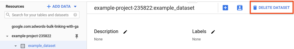
2. In the navigation, select the bqml_tutorial dataset you created.

3. Click Delete dataset on the right side of the window. This action deletes the dataset, the table, and all the data.

   

4. In the Delete dataset dialog box, confirm the delete command by typing the name of your dataset (bqml_tutorial) and then click Delete.

Delete your project

To delete the project:

Caution: Deleting a project has the following effects:

• Everything in the project is deleted. If you used an existing project for the tasks in this document, when you delete it, you also delete any other work you've done in the project.
• Custom project IDs are lost. When you created this project, you might have created a custom project ID that you want to use in the future. To preserve the URLs that use the project ID, such as an appspot.com URL, delete selected resources inside the project instead of deleting the whole project.

If you plan to explore multiple architectures, tutorials, or quickstarts, reusing projects can help you avoid exceeding project quota limits.

1. In the Google Cloud console, go to the Manage resources page.

   Go to Manage resources

2. In the project list, select the project that you want to delete, and then click Delete.
3. In the dialog, type the project ID, and then click Shut down to delete the project.

What's next

• To learn more about machine learning, see the Machine learning crash course.
• For an overview of BigQuery ML, see Introduction to BigQuery ML.
• To learn more about the Google Cloud console, see Using the Google Cloud console.